In this project, I develop a systematic approach to translating the classical three-body problem into a computational framework. The primary objective is to map the initial conditions, gravitational interactions, and subsequent dynamics of three interacting bodies into executable code. I generate phase space trajectories, Poincaré maps, and energy distribution plots to visualize and analyze the chaotic behavior inherent in the three-body system. This approach provides a robust tool for exploring the intricate dynamics of the three-body problem, offering insights into stability, periodicity, and energy interactions. The outcomes of this project lay the groundwork for future research in N-body simulations and the potential development of a compiler to predict complex dynamical behaviors.
Introduction
Introduction
The three-body problem has fascinated scientists since Newtonian times due to its rich and complex dynamics. In a system where three masses interact through gravitational forces, predicting their individual motions over time is non-trivial and leads to chaotic trajectories. The purpose of this project is to create a computational tool that converts the equations governing the three-body problem into executable code. This tool not only simulates the motion of the bodies but also provides analytical tools to study the system’s behavior over extended periods.
This work begins with a review of background material related to the subject starting with the classical three-body problem in Section 1.1, followed by an overview of the equations of motion and the challenges associated with solving them in Section 1.2. Finally, the relevance and importance of computational methods in studying the three-body problem are discussed in Section 1.3. Following, section 2.1 introduces the initial conditions and parameters used in the simulations, including the masses, positions, and velocities of the bodies. Section 2.2 describes the numerical methods employed to integrate the equations of motion over time. Section 2.3 focuses on the visualization techniques used to analyze the system’s behavior. In Section 4, the visualization and animation of three-dimensional trajectories of the bodies are presented, showcasing the dynamic evolution and interaction within the system. These visualizations provide an intuitive understanding of the complex motions and interactions occurring in the three-body problem. Finally, in Section 5, potential directions for future work are outlined.
This work begins with a review of background material related to the subject starting with the classical three-body problem in Section 1.1, followed by an overview of the equations of motion and the challenges associated with solving them in Section 1.2. Finally, the relevance and importance of computational methods in studying the three-body problem are discussed in Section 1.3. Following, section 2.1 introduces the initial conditions and parameters used in the simulations, including the masses, positions, and velocities of the bodies. Section 2.2 describes the numerical methods employed to integrate the equations of motion over time. Section 2.3 focuses on the visualization techniques used to analyze the system’s behavior. In Section 4, the visualization and animation of three-dimensional trajectories of the bodies are presented, showcasing the dynamic evolution and interaction within the system. These visualizations provide an intuitive understanding of the complex motions and interactions occurring in the three-body problem. Finally, in Section 5, potential directions for future work are outlined.
1. Background
1. Background
1.1 The Classical Three-Body Problem
1.1 The Classical Three-Body Problem
The three-body problem involves solving Newton’s equations of motion for three masses that interact through gravitational forces. Given the initial positions and velocities of the bodies, the challenge is to determine their subsequent motion. The complexity of this problem arises from the non-linear nature of gravitational interactions, leading to a system of coupled differential equations that are highly sensitive to initial conditions.
The equations of motion for a three-body system can be expressed as:
The equations of motion for a three-body system can be expressed as:
F
i
m
i
a
i
3
∑
j1j≠i
m
i
m
j
r
j
r
i
-
r
j
r
i
3
|
These equations are coupled and must be solved simultaneously to predict the motion of the bodies. Historically, solutions to the three-body problem have been sought using various analytical and numerical methods, but the inherent chaos and sensitivity to initial conditions make it an extremely challenging problem.
1.2 Equations of Motion and Challenges
1.2 Equations of Motion and Challenges
The chaotic nature of the three-body problem was first rigorously demonstrated by Henri Poincaré in the late 19th century. This sensitivity means that tiny differences in starting conditions can lead to vastly different outcomes, making long-term prediction difficult without exceedingly precise initial data. Traditional numerical methods, such as the Brutus integrator, allow for close-to-zero time-steps and arbitrary precision, but the computational costs can be prohibitive over long time spans due to the rapid divergence of trajectories [1, 2]. Recent advancements have been made to address these challenges, including more sophisticated numerical integrators that aim to maintain accuracy while reducing computational overhead. Despite these advancements, the chaotic behavior of the system often limits the effectiveness of these methods over extended periods.
1.3 Computational Methods and Their Importance
1.3 Computational Methods and Their Importance
In recent years, there has been growing interest in leveraging machine learning and advanced numerical methods to tackle the computational difficulties of the three-body problem. For example, deep artificial neural networks (ANNs) have shown potential in providing accurate solutions at a fraction of the computational cost of traditional methods. These networks can be trained on ensembles of solutions obtained from precise numerical integrators and can subsequently predict trajectories with remarkable speed and accuracy [1, 2]. However, there are differing views on the applicability of these methods. Some suggest that the chaotic nature of the three-body problem limits the effectiveness of machine learning algorithms due to the system' s volatility. The complexity and sensitivity to initial conditions mean that these algorithms may struggle to provide reliable predictions over extended periods [3].
2. Methodology
2. Methodology
2.1 Initial Conditions and Parameters
2.1 Initial Conditions and Parameters
2.2 Simulation
2.2 Simulation
2.3 Visualization
2.3 Visualization
Visualization techniques were used to analyze the system’s behavior, including trajectory plots, phase space diagrams, and energy distribution charts. These visualizations provide insights into the motion and interactions of the bodies over time.
Trajectory Plots
Trajectory Plots
Out[]=

Figure 1: Shows the trajectories of the three bodies within the simulated timeframe. Each body' s path is distinctly colored to highlight their interactions and close encounters.
This provides a clear depiction of how each body moves within the simulated timeframe, highlighting any interactions or close encounters.
Extended Simulation and Analysis
Extended Simulation and Analysis
Phase Space
Phase Space
Out[]=
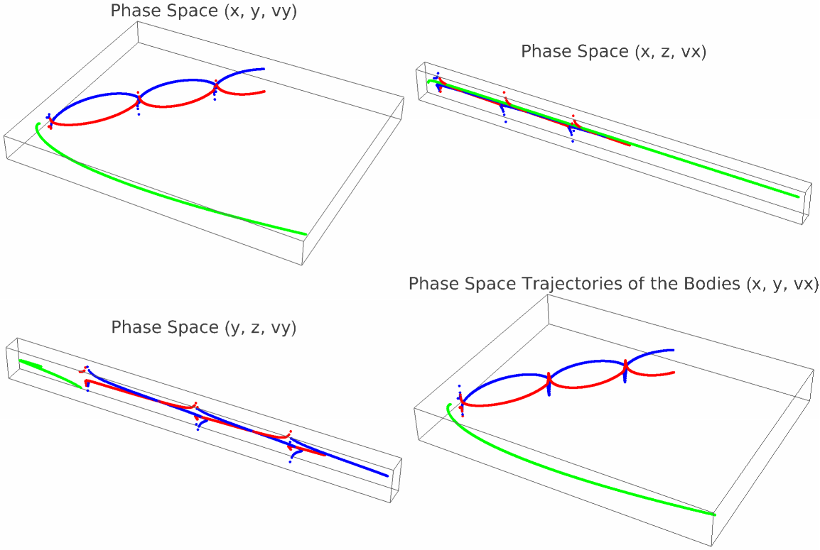
Figure 2: Depicts the phase space of the bodies in various configurations (e.g., x, y, vy and x, z, vx) These diagrams illustrate the system's behavior in different coordinate spaces, revealing patterns in the velocity and position of the bodies [4].
Energy Analysis
Energy Analysis
Out[]=
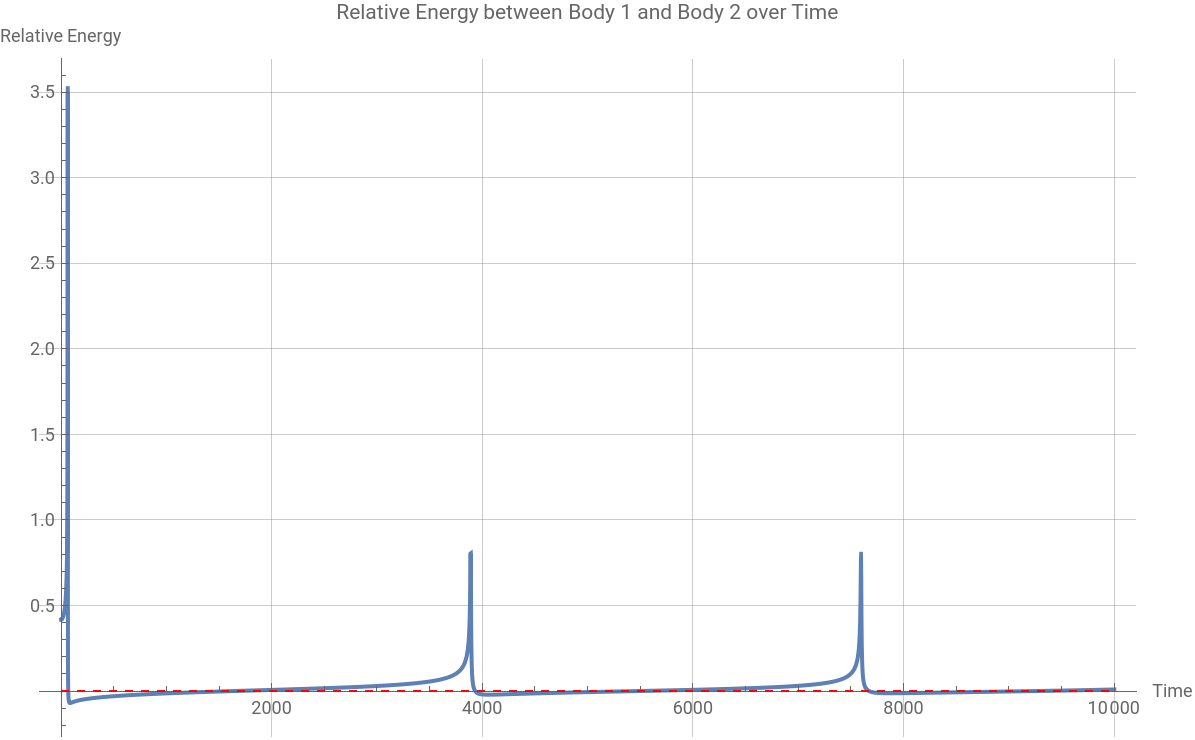
Figure 3: The relative energy between Body 1 and Body 2 over time.
The periodic peaks in the energy values indicate regular exchanges between kinetic and potential energy, characteristic of the gravitational interactions among the bodies. The kinetic energy shows distinct spikes at regular intervals, corresponding to points where the bodies come closest together, while the potential energy exhibits corresponding dips.
Binding Status Analysis
Binding Status Analysis
Out[]=
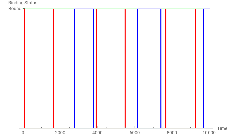


Figure 4: The gravitational binding between different pairs of bodies over time. Periodic binding and unbinding events are highlighted, indicating the fluctuating nature of their interactions.
Body 1 and Body 3 remain consistently bound throughout the simulation, as indicated by the green line maintaining a constant value of 1. This suggests a stable gravitational interaction between these two bodies, likely due to their initial conditions and relative velocities ensuring a persistent binding. In contrast, the binding status between Body 1 and Body 2, and between Body 2 and Body 3, exhibits periodic changes, as shown by the alternating segments of 1 and 0 in the red and blue lines, respectively. These fluctuations indicate that these pairs experience phases where they are gravitationally bound, interspersed with intervals where they are not. This dynamic behavior is characteristic of the three-body problem, where complex gravitational interactions lead to non-linear and often chaotic motion. The periodic binding and unbinding suggest that the relative distances and velocities between these bodies vary significantly over time, causing intermittent gravitational capture and release.
Poincaré Maps
Poincaré Maps
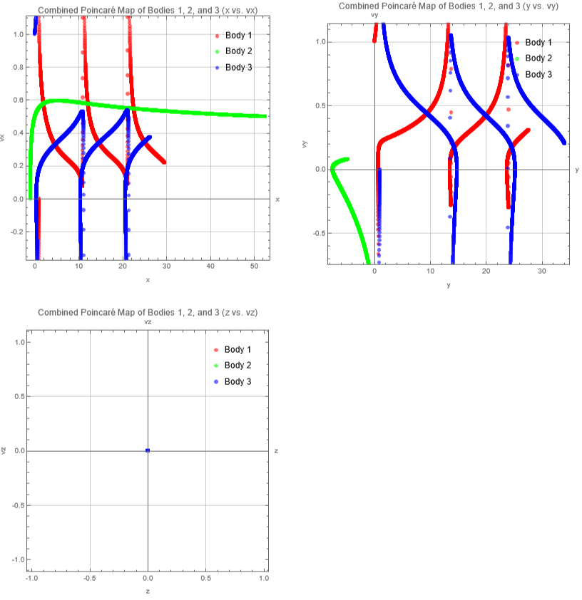
Figure 5: Poincaré maps for different coordinate spaces.
Fig. 5a shows the combined Poincaré map for Bodies 1, 2, and 3 in the x vs. vx
space, revealing distinct clusters and periodic patterns that indicate regions of frequent returns and chaotic dynamics. Body 1 (red) and Body 3 (blue) exhibit more complex trajectories, while Body 2 (green) shows more regular motion. Fig. 5b presents the combined Poincaré map for Bodies 1, 2, and 3 in the y vs. vy space, displaying similar periodic clusters and chaotic interactions, particularly for Bodies 1 and 3, with Body 2 again demonstrating a relatively regular trajectory. Fig. 5c, the combined Poincaré map for Bodies 1, 2, and 3 in the z vs. vz space, appears empty, suggesting minimal variation or interaction in the z-direction for the given initial conditions and velocities, implying that the primary dynamics of the system are constrained within the x-y plane, with negligible motion along the z-axis.
space, revealing distinct clusters and periodic patterns that indicate regions of frequent returns and chaotic dynamics. Body 1 (red) and Body 3 (blue) exhibit more complex trajectories, while Body 2 (green) shows more regular motion. Fig. 5b presents the combined Poincaré map for Bodies 1, 2, and 3 in the y vs. vy space, displaying similar periodic clusters and chaotic interactions, particularly for Bodies 1 and 3, with Body 2 again demonstrating a relatively regular trajectory. Fig. 5c, the combined Poincaré map for Bodies 1, 2, and 3 in the z vs. vz space, appears empty, suggesting minimal variation or interaction in the z-direction for the given initial conditions and velocities, implying that the primary dynamics of the system are constrained within the x-y plane, with negligible motion along the z-axis.
Detailed analysis of the Poincaré maps provides a powerful tool for visualizing the periodicity and chaotic behavior of the system, offering deeper insights into the underlying dynamics of the three-body problem [5, 6].
Detailed Energy Analysis
Detailed Energy Analysis
Figure 6: The exchanges between kinetic and potential energy for different pairs of bodies.
Fig. 6a depicts the energy distribution between Body 1 and Body 2, where periodic spikes in kinetic energy correspond to points where the bodies come closest together, while potential energy dips indicate increased gravitational attraction. Figure 6b presents the energy distribution between Body 1 and Body 3, showing similar periodic patterns with regular exchanges between kinetic and potential energy. Figure 6c illustrates the energy distribution between Body 2 and Body 3, which exhibits less frequent but still significant energy exchanges. The periodic nature of the peaks and troughs in these figures indicates regular energy transfers, characteristic of the gravitational interactions among the bodies. These patterns provide insights into the stability and dynamical behavior of the three-body system, revealing the interplay between kinetic and potential energy as the bodies interact over time.
Perturbation Analysis
Perturbation Analysis
Figure 7: The energy perturbations between pairs of bodies, highlighting the influence of the third body’s gravitational force on the energy exchanges.
Fig. 7a shows the perturbations between Body 1 and Body 2 due to the influence of Body 3, with periodic peaks and troughs indicating moments of significant energy exchange. Fig. 7b presents similar perturbations between Body 1 and Body 3 due to Body 2, displaying a pattern of periodic energy fluctuations. Fig. 7c depicts the perturbations between Body 2 and Body 3 influenced by Body 1, showing a more complex and asymmetric pattern of energy exchange. These plots reveal that the third body’s gravitational force intermittently perturbs the energy balance within each pair, resulting in non-symmetric fluctuations. This asymmetry is indicative of the dynamic and complex nature of three-body interactions, where the gravitational influence of each body continually alters the energy states of the others. The periodicity and amplitude of these perturbations provide insights into the timing and intensity of the interactions, revealing the intricate dance of gravitational forces within the system.
4. Code Compilation and Execution
4. Code Compilation and Execution
In this section, the focus is on transforming the simulation results into executable code, effectively compiling the system’s state into a computationally interpretable format. This approach aims to bridge the gap between theoretical simulations and practical implementations.
Three-Dimensional Trajectories
Three-Dimensional Trajectories
Figure 8: Three-Dimensional Trajectories – visualization of the trajectories of three interacting bodies in a 3D space.
This section highlights the practical application of the computational methods used in this project, emphasizing the potential for developing tools to predict complex dynamical behaviors in N-body simulations.
5. Concluding Remarks
5. Concluding Remarks
This computational exploration of the three-body problem has provided a comprehensive view of how these bodies move and interact over time. The trajectories reveal the paths each body takes, showing their close encounters and mutual influences. The phase space analysis, with both combined and separate Poincaré maps, illustrates repeating patterns and chaotic behavior. Bodies 1 and 3 exhibit more complex interactions, while Body 2 follows a smoother path, indicating a diverse range of dynamical behaviors within the system.
The energy analysis demonstrates regular exchanges between kinetic and potential energy. Kinetic energy peaks and potential energy dips when the bodies come close, indicating a consistent energy exchange pattern. This regular exchange shows that while the total energy is conserved, it continually shifts between kinetic and potential forms. The perturbation analysis further highlights the impact of the third body’s gravitational influence on the energy balance within each pair. Periodic peaks and drops in energy suggest significant energy changes caused by the third body, underscoring the complex and dynamic nature of their interactions.
The energy analysis demonstrates regular exchanges between kinetic and potential energy. Kinetic energy peaks and potential energy dips when the bodies come close, indicating a consistent energy exchange pattern. This regular exchange shows that while the total energy is conserved, it continually shifts between kinetic and potential forms. The perturbation analysis further highlights the impact of the third body’s gravitational influence on the energy balance within each pair. Periodic peaks and drops in energy suggest significant energy changes caused by the third body, underscoring the complex and dynamic nature of their interactions.
Future Work
Future Work
◼
Two - Body Interaction Collision with Third Body : Investigate the dynamics when two bodies collide with the third body, including the impact parameter . This could reveal persistent structures useful for building a “compiler” to predict complex behaviors .
◼
Extended Simulation Timeframes: Increase the duration of simulations to observe long-term behaviors and stability in the system, potentially uncovering new dynamical regimes.
◼
Variable Masses and Initial Conditions: Study the effects of varying masses and different initial conditions to understand how these factors influence the overall dynamics and stability of the system.
◼
Incorporation of External Forces: Introduce external forces, such as tidal forces or relativistic effects, to simulate more realistic astrophysical scenarios.
◼
Higher-Dimensional Analysis: Extend the analysis to higher dimensions, examining the system’s behavior in additional spatial dimensions or considering more bodies in the simulation
Acknowledgments
Acknowledgments
I would like to express my heartfelt appreciation to my mentors, Paul Abbott, John McNally, and Vladimir Grankovsky, for their support and insightful guidance throughout this project. Additionally, I extend my gratitude to the administrators, speakers, and TAs at Wolfram Summer School 2024 for creating an enriching and inspiring environment. A special thank you to Stephen Wolfram for his visionary ideas and suggestions that inspired this work.
References
References
1
.Philip G. Breen, Christopher N. Foley, Tjarda Boekholt, and Simon Portegies Zwart (2019), “Newton vs the machine: solving the chaotic three-body problem using deep neural networks,” arXiv. https://arxiv.org/abs/1910.07291
2
.William Ditto, Kotra Murali, and Sudeshna Sinha (2007), “Chaos computing: Ideas and implementations,” Philosophical Transactions A. https://www.researchgate.net/publication/6142096_Chaos_computing_Ideas_and_implementations
3
.Pedro Cabral (2019), “Patterns in N-Body Simulations: Analysis of the Three Body Problem,” Wolfram Community. https://community.wolfram.com/groups/-/m/t/1731612
4
.Barak Kol (2021), “Flux-based statistical prediction of three-body outcomes,” Celestial Mechanics and Dynamical Astronomy. https://link.springer.com/article/10.1007/s10569-021-10015-x
5
.Nicholas C. Stone and Nathan W. C. Leigh (2019), “A statistical solution to the chaotic, non-hierarchical three-body problem,” Nature. https://www.nature.com/articles/s41586-019-1833-8
Cite This Notebook
Cite This Notebook