Introduction to Billiard Polygons
Introduction to Billiard Polygons
Billiards are dynamical systems where particles alternate from motion in a straight line to reflections at a boundary. The traditional problem consists of a piecewise-linear 2D boundary region containing a single moving particle. Polygonal billiards are constrained by a boundary with vertex angles that are rational multiples of π.
A game of billiards is typically played on a rectangular table with six pockets. Arithmetic or mathematical billiards simplify this idea by disregarding any pockets and friction between the “ball” and the “table”. Unlike a traditional game of billiards where there are many balls, this simulation only has one particle. The ball bounces around according to the same rules as an ordinary ball, moving along a straight line until it hits the edge of the boundary (in this case, a regular polygon) where it bounces off following the law of reflection. This particle has neither mass nor friction and continues indefinitely with its progress measured in "time steps" (each line segment preceding a reflection). If the particle enters one of the vertices of the polygon, the simulation will halt because its next action is unpredictable.
The purpose of this project was to computationally analyze the billiard polygons and to characterize the density and ergodicity of this system under varying initial conditions.
Methods
Methods
Creating the Billiard Polygons
Creating the Billiard Polygons
The Wolfram Language has a resource function called BilliardPolygon that allows you to change many features (initial position, angle, etc.) to create a graphic displaying the path of the particle for a specified amount of time steps. I experimented with different iterations of time steps and tested different initial angles and positions using this function. I also created a simple function using Manipulate to see the graphics in real time over the specified number of time steps. These are a few examples of the very first lines of code that I experimented with to understand the properties of this large resource function:
In[]:=
GraphicsGrid[{Table[ResourceFunction["BilliardPolygon"][n,{.01,.1},Pi/3, 300],{n,3, 10}]}, ImageSize2300]
Out[]=

In[]:=
Manipulate[Grid@Table[Graphics[ResourceFunction["BilliardPolygon"][n+j,{.01,.1},Pi/3,steps],ImageSize1000],{j,1,1},{n,2,8}],{steps,1,300}]
Characterizing Density and Ergodicity
Characterizing Density and Ergodicity
What do density and ergodicity mean in this scenario?
What do density and ergodicity mean in this scenario?
For the purpose of the current simulation, density refers to the "filling in" of the polygon by the lines representing the path of the particle. For some initial conditions, a particular path will be traversed several times by the particle as it retraces its previous traversals. In other cases, the particle will cover more of the surface of the polygon as it bounces against the boundaries resulting in a higher density. In my simulations, the path is represented by lines of fixed width and more pixels are filled in when the path is nonperiodic.
When the particle retraces its path over a fixed number of steps, the ratio of filled pixels to the total number of pixels representing the polygon remains low and the path is considered to be ergodic since the particle eventually returns to its initial state. At this point, increasing the number of steps in the simulation results in no additional filling and I used this property to characterize certain paths as ergodic. For a large fixed number of steps, I classified particles with low final filling ratios (density) as ergodic.
When the particle retraces its path over a fixed number of steps, the ratio of filled pixels to the total number of pixels representing the polygon remains low and the path is considered to be ergodic since the particle eventually returns to its initial state. At this point, increasing the number of steps in the simulation results in no additional filling and I used this property to characterize certain paths as ergodic. For a large fixed number of steps, I classified particles with low final filling ratios (density) as ergodic.
Exploring Different Graphics Methods
Exploring Different Graphics Methods
For my initial approach, I used a series of image processing manipulation functions such as Binarize and ImageLevels to convert the image into a format facilitating the calculating of pixel density. This is one example of the types of trials I used to test these functions:
In[]:=
Binarize[Part[Image[Table[ResourceFunction["BilliardPolygon"][n,{.7,.1},Pi/12,900],{n,3,3}]],1]]pixels = ImageLevels[Binarize[Part[Image[Table[ResourceFunction["BilliardPolygon"][n,{.7,.1},Pi/12,900],{n,3,3}]],1]]]
This is one method of generating the number of white and black pixels in the figure in order to calculate the filling ratio (density). I ended up not using this exact approach because I was eventually able to use a more accurate approach to discretize the polygon image using ImageData (see below).
Edited Billiard Polygon Resource Function
Edited Billiard Polygon Resource Function
Since BilliardPolygon was the basis of my simulations, I needed to make a few changes to adapt the function for my ergodicity analysis. :
◼
Removal of the border features: In the original function, a green line was implemented using RGBColor and Thickness. To calculate the fill ratio more accurately, the border color was changed to black and the thickness was reduced. The border pixels were removed during the density calculation to avoid including the perimeter of the polygon.
◼
Angle offset: The output of BilliardPolygon demonstrated a slight rotation in the polygon to avoid numerical issues resulting from particles entering a vertex. As an example, if the polygon had not been rotated in this manner, a particle starting at the center with an initial angle of zero would head straight for the vertex at (0,1). For this reason, BilliardPolygon employed and angle offset of 0.1 radians. I converted this hardcoded constant into a variable so I could account for it in my calculations.
BilliardPolygonTST[sides_,start_,angle_,n_, angleoffset_]:=Module[{impderiv,corners,cushions,slopes,pos,dir,traj,slope,path,solns,solnrules,hit,eps=10^(-10),lineFromCorners},impderiv[{x1_,y1_}]:=slopes[[Position[(First[#1]-Last[#1]&)/@cushions/.Thread[{x,y}{x1,y1}],_?(Abs[#1]<eps&)][[1,1]]]];lineFromCorners[{p1:{x1_,y1_},p2:{x2_,y2_}}]:=With[{aslope=Divide@@Reverse[p1-p2]},yy1+aslope*(x-x1)];corners=Partition[({Cos[#1],Sin[#1]}&)/@Range[angleoffset,2*Pi + angleoffset,2*(Pi/sides)],2,1];slopes=(Divide@@Reverse[#1[[1]]-#1[[2]]]&)/@corners;cushions=lineFromCorners/@corners;traj={pos=start};slope=Tan[dir=angle];path=y-pos[[2]]slope*(x-pos[[1]]);solnrules=Solve[{path,Or@@cushions},{x,y}];solns=Select[{x,y}/.solnrules,Plus@@(#1^2)≤1.&];hit=Select[solns,And@@Thread[#1>pos]&];AppendTo[traj,hit[[1]]];Do[slope=Tan[2*Pi-(ArcTan@@(hit[[1]]-pos)-ArcTan[impderiv[hit[[1]]]])+ArcTan[impderiv[hit[[1]]]]];pos=hit[[1]];path=y-pos[[2]]slope*(x-pos[[1]]);solnrules=Solve[{path,Or@@cushions},{x,y}];solns=Select[{x,y}/.solnrules,Plus@@(#1^2)≤1.&];hit=Select[solns,(#1-pos).(#1-pos)>eps&];AppendTo[traj,hit[[1]]],{n}];Graphics[{{Line[({Cos[#1],Sin[#1]}&)/@Range[angleoffset,2*Pi+angleoffset,2*(Pi/sides)]]},Line[traj]},AspectRatioAutomatic,FrameFalse,AxesFalse,ImageSize{400,400}]]angoffset = 0.1
Exploring the Effect of Polygon Shape
Exploring the Effect of Polygon Shape
When the same initial angle (π/4) is used for polygons of different shapes, a variety of interesting patterns can be seen, some of which are clearly ergodic. In particular, if the polygon has number of sides equivalent to a multiple of four, the pattern is ergodic with a period of two. This is not seen in the polygon with eight and sixteen sides since using this angle results in the particle going straight into a vertex.
In[]:=
Quiet[Table[BilliardPolygonTST[n,{0,0},Pi/4 + angoffset, 100, angoffset],{n,3,20}]]
Geometric Characterization of Polygons
Geometric Characterization of Polygons
The number of sides of the simulated polygon can be used to calculate its InternalAngle. The maxangle was chosen to be half of the internal angle and was used as the maximum angle in all of the simulations below. The vertexangles illustrated in the figure below, was used to calculate the coordinates of the vertices (coords). The vertexangles variable represents the angle from the origin to the vertex.
In[]:=
n=4 (* Number of sides *)InternalAngle[n_] := Pi-2Pi/nmaxangle = (Pi - InternalAngle[n])/2vertexangles = Table[i,{i,0,n}]*(2Pi/n) + angoffsetcoords = Transpose[{Cos[vertexangles],Sin[vertexangles]}]
As an example, the four sided regular polygon below (as displayed in accordance with BilliardPolygon rotated by 0.1 radians) is shown inscribed in the unit circle.
In[]:=
Show[{ListLinePlot[coords],PolarPlot[1,{theta,0,2Pi}]}, AspectRatio1]
Out[]=
Generating a Basic Ergodic Pattern by Connecting Midpoints
Generating a Basic Ergodic Pattern by Connecting Midpoints
The midpoints of each side of the polygon can be calculated by averaging the vertex coordinates.
In[]:=
midpoints = Table[(coords[[1+Mod[i,n]]]+coords[[1+Mod[i+1,n]]])/2,{i,0,n}]
Connecting the midpoints results in a regular inscribed polygon within the original polygon.
In[]:=
Show[{ListLinePlot[{coords, midpoints}],PolarPlot[1,{theta,0,2Pi}]}, AspectRatio1]
Out[]=
The variable midpointangles represents the angle from the midpoint of one line segment to the midpoint of the next line segment.
midpointangles= Table[VectorAngle[midpoints[[i+1]]-midpoints[[i]],{1,0}],{i,1,n}](* midpointangles = Table[ArcTan[-Part[midpoints[[i+1]]-midpoints[[i]],2]/Part[midpoints[[i+1]]-midpoints[[i]],1]],{i,1,n}] *)(* midpointangles = Table[VectorAngle[coords[[i+1]]-coords[[i]],{1,0}],{i,1,n}] *)midpoints[[n-1]]
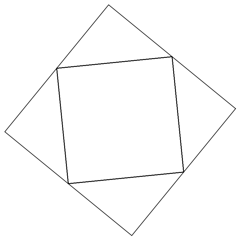
Using this angle as the initial angle in BilliardPolygon generates an ergodic pattern with a period equal to the number of sides.
In[]:=
Quiet[BilliardPolygonTST[n,midpoints[[n-1]],midpointangles[[n-1]], 100, angoffset]]
Out[]=
Systematic Exploration of Particle Angle Variation on Fill Density
Systematic Exploration of Particle Angle Variation on Fill Density
I then systematically explored the effect of change in the initial angle for a particle starting at the origin in regular polygons of different shapes. Image analysis as described above was used to calculate the fill ratios (i.e. the density) of the polygons after a fixed number of time steps. This filling density was used as a surrogate measure of ergodicity, with lower fill ratios representing more ergodic trajectories. The maximum angle used was half of the internal angle since the results be expected to be symmetric over the entire range of internal angle.
Characterizing Density with a Uniform Distribution of Angles
Characterizing Density with a Uniform Distribution of Angles
Fill ratios were calculated for a range of angles from zero to maxangle first by using a uniform distribution of angles. Ergodicity was not expected in most cases because these ratios did not necessarily represent ratios of small integers.
Once this table was generated, the following commands were used to visualize the data:
Characterizing Density with Only Rational Initial Angles
Characterizing Density with Only Rational Initial Angles
Next, fill ratios were calculated for ratios of small integers (rational numbers) in the range of zero to one. Once this list was constructed, these multiples of maxangle were used to create a table that was used to calculate fill ratios.
The ratios generated were not in numerical order but are represented accurately when plotted against the resulting densities. The table of densities generated from these maxangle ratios was plotted in a similar manner to the graphs using a uniform angle distribution.
Results
Results
The graphs in this section represent a sampling of density results for polygons of sides 3 to 7. For each polygon, both uniform and rational initial angle ratios were considered. The range of angles was normalized by maxangle such that the angle distributions shown below range from zero to one. The fill ratios calculated were displayed as density fractions also ranging from zero to one. Accompanying histograms show the frequency distributions for density in both cases (uniform and rational angle distributions).
Equilateral triangle, 100 angles between 0 and π/6, 100 time steps, initial position of the particle: (0,0)
Uniform:
Rational:
Square, 100 angles between 0 and π/4, 100 time steps, initial position of the particle: (0,0)
Uniform:
Rational:
Regular pentagon, 100 angles between 0 and 3π/10, 100 time steps, initial position of the particle: (0,0)
Uniform:
Rational:
Regular hexagon, 100 angles between 0 and π/3, 100 time steps, initial position of the particle: (0,0)
Uniform:
Rational:
Regular heptagon, 100 angles between 0 and 5π/14, 100 time steps, initial position of the particle: (0,0)
Uniform:
Rational:
The range of angles simulated shows a wide fluctuation in polygon fill ratios, suggesting that changing the angle even slightly can result in nonoverlapping paths. Lower fill ratios for large numbers of iterations suggest paths that are repeatedly followed and can be characterized as ergodic. Angles resulting in ergodic behavior can be found scattered among highly nonergodic angles. Even using a list of rational numbers to construct initial angles generated nonergodic patterns in many instances, suggesting that a more complicated relationship may exist. This is similar to other dynamical systems in which small changes in particles’ initial conditions can result in large differences in their trajectories.
One feature evident in the graphs above is the bimodal frequency distribution of densities as the angle is varied. This suggests a clear distinction between ergodic and nonergodic initial angles. In the cases where rational angle ratios were used, the distribution is especially bimodal suggesting that more of these cases were strongly ergodic. (Note in particular the isolated ergodic angles found in the lower region of the rational heptagon case.) The fact that many rational angles still led to high fill ratios suggests that even small integer ratios of initial angle are not guaranteed to be ergodic.
One feature evident in the graphs above is the bimodal frequency distribution of densities as the angle is varied. This suggests a clear distinction between ergodic and nonergodic initial angles. In the cases where rational angle ratios were used, the distribution is especially bimodal suggesting that more of these cases were strongly ergodic. (Note in particular the isolated ergodic angles found in the lower region of the rational heptagon case.) The fact that many rational angles still led to high fill ratios suggests that even small integer ratios of initial angle are not guaranteed to be ergodic.
Conclusion
Conclusion
From the results, it can be concluded that ergodicity demonstrates complex behavior and seems to have an enigmatic relationship with rational numbers that deserves to be explored more fully in the future. The density (as measured by fill ratio) was extremely sensitive to the angle, and my results demonstrate the presence of many low density values scattered through the angle range which represent periodic patterns and are therefore ergodic. Because polygon filling can vary wildly from one angle to the next, this behavior can be characterized as chaotic and could potentially be analyzed further using dynamical systems theory. These investigations might provide some insight into the numerical principles of mathematical billiards and their applications.
Future Work
Future Work
In the future, I plan to test regular polygons of higher numbers of sides to see what patterns may arise. Another approach to determine particle reflections at the boundary, would be using some sort of intersection function which detects when the particle reaches the perimeter of the polygon. A transform function to find the peaks and valleys in the density graphs may reveal patterns of ergodicity as the initial angle is varied. I would also like to explore different ways of visualizing the data which may provide additional insights into situations where the patterns are ergodic. Another way to characterize ergodicity besides pixel density and image analysis may be to consider the period of repetitive paths (i.e the length of each cycle) before the particle returns to its initial state. The method of unfolding would also provide an alternative to determining reflection at the boundary instead of simulating particle motion. Simulating irregular polygons such as parallelograms would require entirely rewriting the resource function BilliardPolygon, which may also produce some interesting and different results. Finally, it would also be interesting to simulate many particles and curved boundaries and to simulate collisions between particles.
Full Code
Full Code
References
References
◼
Baez, J. (2016). Bunimovich stadium. American Mathematical Society. Taken from: https://blogs.ams.org/visualinsight/2016/11/15/bunimovich-stadium/
◼
Freiberger, M. (2014). Chaos on the billiard table. +Plus Magazine…Living Mathematics. Taken from: https://plus.maths.org/content/chaos-billiard-table
◼
Kokshenev, V. (2005). On chaotic dynamics in rational polygonal billiards. Symmetry, Integrability and Geometry: Methods and Applications. 1(014).1-9.
◼
Masur, H. & Tabachnikov, S. (1999). Rational billiards and flat structures. University of Chicago. Taken from: https://www.math.uchicago.edu/~masur/handbook1.pdf
◼
Mathematics. (2010). Polygonal billiards and uniform distribution. Taken from: https://math.stackexchange.com/questions/6038/polygonal-billiards-and-uniform-distribution
◼
MathOverflow. (2014). Existence of nonergodic polygonal billiard. Taken from: https://mathoverflow.net/questions/163634/existence-of-nonergodic-polygonal-billiard
◼
Troubetzkoy, S. & Hubert, P. (2000). Polygonal billiards: Some open problems. Institut de Mathematiques de Luminy. Taken from: https://www.math.iupui.edu/~mmisiure/open/ht1.pdf
◼
Zemlyakov, AN & Katok, AB. (1975). Topological transitivity of billiards in polygons. Mathematical notes of the Academy of Sciences of the USSR. 18, 760-764.