This notebook tackles the problem of changing variables in general stochastic differential equations (SDEs) for both Stratonovich and Ito processes. We utilize two custom functions to investigate key examples and physical applications, highlighting the capability to apply named coordinate transformations and explicitly inspect the resulting symbolic terms.
Function repository functions
Function repository functions
Regarding the details of how the transformations are done , it is advised to check the documentation of the Wolfram Function Repository:
For Stratonovich processes:
In[]:=
ResourceFunction["StratonovichProcessChangeVariables"]
Out[]=
For Ito processes:
In[]:=
ResourceFunction["ItoProcessChangeVariables"]
Out[]=
Change of variables for a Stratonovich process
Change of variables for a Stratonovich process
Use cases
Use cases
Square transformation
Square transformation
Define a Stratonovich process:
In[]:=
procX=StratonovichProcess1,σExp[-],{x,x0},t
2
x
2
x
Out[]=
StratonovichProcess,σ,x[t],{{x},{x0}},{t,0}
1
2
x[t]
-
2
x[t]
Square transformation of the process:
In[]:=
transformed=[procX,y,y==x^2];
Check is a valid process:
In[]:=
ProcessParameterQ[transformed]
Out[]=
True
Print the transformed drift and diffusion terms:
In[]:=
Print["Drift: ",transformed["Drift"],"\nDiffusion: ",transformed["Diffusion"]]
Drift: -Diffusion: -2σ
2
y[t]
-y[t]
y[t]
Cubic transformation of a Wiener process
Cubic transformation of a Wiener process
Start with a Stratonovich process that has a Wiener process form:
In[]:=
proc=StratonovichProcess[{0,1},{x,x0},t]
Out[]=
StratonovichProcess[{{0},{{1}},x[t]},{{x},{x0}},{t,0}]
Cubic transformation of a process:
In[]:=
Out[]=
StratonovichProcess{0},3,y[t],{{y},{}},{t,0}
2/3
y[t]
3
x0
Time scaling
Time scaling
Start with a general process with drift a and diffusion b:
In[]:=
spLinear=StratonovichProcess[{a,b},{x,x0},{t,t0}]
Out[]=
StratonovichProcess[{{a},{{b}},x[t]},{{x},{x0}},{t,t0}]
Process variable scaling:
In[]:=
resTimeDep=spLinear,{y},y
x
t
Out[]=
StratonovichProcess,,{y[t]},{y},,{t,0}
a-y[t]
t
b
t
x0
t0
Zero drift process from Ornstein-Uhlenbeck
Zero drift process from Ornstein-Uhlenbeck
Define the following OrnsteinUhlenbeck process:
In[]:=
ou=StratonovichProcess@OrnsteinUhlenbeckProcess[μ,σ,θ,x0]
Out[]=
StratonovichProcessθ(μ-x.[t.]),{{σ}},x.[t.],{{x.},{x0}},t.,0
Consider the transformation y = (x-μ) that is time dependent:
θt
ⅇ
In[]:=
transformed=ou,y,y(x.-μ);
θt.
Check the process is drift-less for this transformation:
In[]:=
transformed["Drift"]=={0}
Out[]=
True
Tangent/Cauchy transformation
Tangent/Cauchy transformation
Start with a Stratonovich process that has form of Wiener process:
In[]:=
procX=StratonovichProcess[{0,1},{x,0},t];
Perform the transformation :
y=Tan(x)
In[]:=
Out[]=
StratonovichProcess[{{0},{{}},y[t]},{{y},{0}},{t,0}]
2
Sec[ArcTan[y[t]]+π]
1
Specify a solving branch for :
0<=x<2π
In[]:=
procY=[procX,y,y==Tan[x],Assumptions->{0<=x<2π}]
Out[]=
StratonovichProcess[{{0},{{1+}},y[t]},{{y},{0}},{t,0}]
2
y[t]
Cylindrical to spherical coordinates
Cylindrical to spherical coordinates
Define a process in cylindrical coordinates:
In[]:=
proc3D=StratonovichProcess[{{1/ρ,0,0},{σ/(ρ^2+z^2),0,σz}},{{ρ,ϕ,z},{ρ0,ϕ0,z0}},t]
Out[]=
StratonovichProcess,0,0,+,{0},{σz[t]},{ρ[t],ϕ[t],z[t]},{{ρ,ϕ,z},{ρ0,ϕ0,z0}},{t,0}
1
ρ[t]
σ
2
z[t]
2
ρ[t]
Perform a transformation to spherical coordinates using long names notation:
In[]:=
Out[]=
StratonovichProcess,,0,σr[t]+,σCosθ.[t]-Sinθ.[t],{0},r[t],θ.[t],φ[t],r,θ.,φ,+,ArcTan[z0,ρ0],ϕ0,{t,0}
1
r[t]
Cotθ.[t]
2
r[t]
2
Cosθ.[t]
σSinθ.[t]
2
r[t]
1
3
r[t]
2
z0
2
ρ0
Physics applications
Physics applications
Stochastic 2D trapping motion
Stochastic 2D trapping motion
Define a stochastic process representing harmonic oscillator trap(including a magnetic effect) in Cartesian coordinates:
In[]:=
spMagnetic=StratonovichProcess[{{-γx+By,-γy-Bx},{{σ,0},{0,σ}}},{{x,y},{x0,y0}},t]
Out[]=
StratonovichProcess[{{-γx[t]+By[t],-Bx[t]-γy[t]},{{σ,0},{0,σ}},{x[t],y[t]}},{{x,y},{x0,y0}},{t,0}]
Change to polar coordinates that are more suitable to the problem:
In[]:=
spPolar=[spMagnetic,{r,ϕ},"Cartesian"->"Polar"]
Out[]=
StratonovichProcess{-γr[t],-B},{σCos[ϕ[t]],σSin[ϕ[t]]},-,,{r[t],ϕ[t]},{r,ϕ},+,ArcTan[x0,y0],{t,0}
σSin[ϕ[t]]
r[t]
σCos[ϕ[t]]
r[t]
2
x0
2
y0
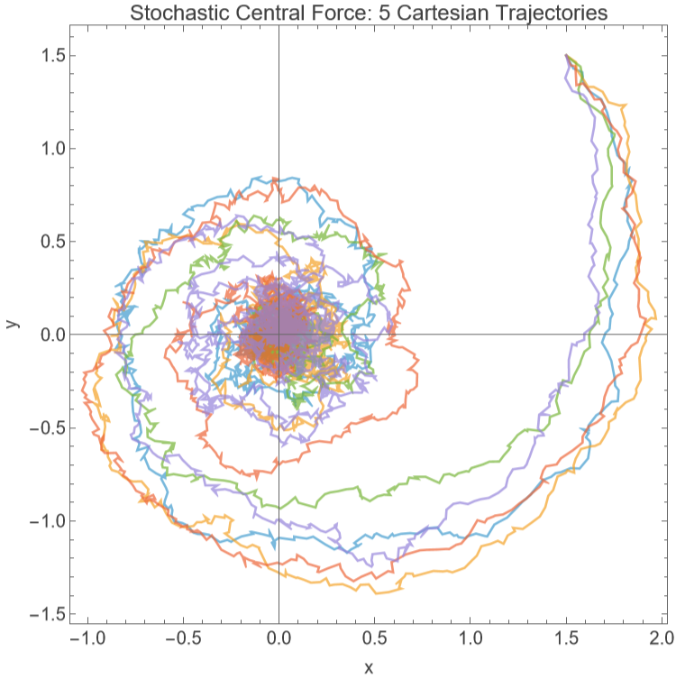
Set up parameters and simulate 5 paths:
In[]:=
paths=RandomFunction[spPolar/.{γ->0.5,B->2,σ->0.2,x0->1.5,y0->1.5},{0,20,0.01},5];
Swap back to Cartesian coordinates for plotting:
In[]:=
cartesianPaths=TimeSeriesMap[{#[[1]]Cos[#[[2]]],#[[1]]Sin[#[[2]]]}&,paths];
Plot the paths:
In[]:=
ListLinePlotcartesianPaths["ValueList"],
Out[]=
Cellular flow with diffusion
Cellular flow with diffusion
Define a Stratonovich process representing flow of particles specified by the drift with added thermal fluctuations:
Visualize stream plot of the drift:
Transformed u-v drift stream plot:
Visualize 10 trajectories in the u-v space:
Change of variables for an Ito process
Change of variables for an Ito process
Use cases
Use cases
Log transform of a geometric Brownian motion process
Log transform of a geometric Brownian motion process
Build an Ito process from a Brownian motion stochastic process:
Get the arithmetic Brownian motion via a logarithmic transformation:
Show the PDF of the process:
Exponential transformation
Exponential transformation
Define an Ito process representing a Wiener process:
Perform an exponential transformation:
Mean and variance of the process:
We can get equivalent result for the mean and variance of the process using TransformedProcess:
Mean shifting an Ornstein-Uhlenbeck process
Mean shifting an Ornstein-Uhlenbeck process
Define the OrnsteinUhlenbeck process:
Compute mean and variance of the process:
Check the mean and variance, the mean got shifted but the process remains OrnsteinUhlenbeck:
Using TransformedProcess:
Polar coordinates
Polar coordinates
Start with a 2D Wiener process:
Transform the process to polar coordinates. We see the initial zero drift becomes non zero and only radial dependent in polar coordinates:
Time dependent transformation
Time dependent transformation
Create a particular Ito process:
Explicit time-dependent transformation:
Hyperbolic tangent change of variable
Hyperbolic tangent change of variable
Start with a driftless process:
Cosine transformation
Cosine transformation
Define a 1D Wiener process:
Perform a trigonometric change of variables, because of the periodic nature of the transformation is not possible to get a unique solution:
Physics applications
Physics applications
Harmonic oscillator with noise
Harmonic oscillator with noise
Define a process representing position and velocity of some particle, with drift in velocity related to position (as in Hooke's law). With added diffusion only in the velocity:
Transforming to E and ϕ variables (energy and phase), we are assuming unit mass:
Set up parameters:
Plotting the phase portrait we get deformed circular paths:
Visualizing the paths in energy-phase space using the same parameters, the dashed line is the energy without noise:
Quantum state diffusion
Quantum state diffusion
Perform change of variables to spherical coordinates which are more appropriate to the geometry of the state space:
Calculate Bloch vector trajectories in Cartesian coordinates:
The quantum probabilities from Born rule can be obtained with a histogram of the z component of the Bloch vector for many trajectories , assuming that the time is long enough to produce eigenstate collapse
CITE THIS NOTEBOOK
CITE THIS NOTEBOOK
Change of state variables for general stochastic processes
by Bruno Tenorio
Wolfram Community, STAFF PICKS, January 20, 2026
https://community.wolfram.com/groups/-/m/t/3609731
by Bruno Tenorio
Wolfram Community, STAFF PICKS, January 20, 2026
https://community.wolfram.com/groups/-/m/t/3609731