ABSTRACT (original article): We consider a modified version of the well-known 2d vdP oscillator with a new non-Hermitian interaction. The usual perturbative approach fails to provide the classical dynamics of the system as the classical solutions become divergent in the long time limit. These kinds of divergences are similar to what occurs in quantum field theory and critical phenomena. The Renormalization Group (RG) technique for the dynamical system has been used to eliminate the divergences in the perturbative solution of the 2d vdP oscillator and to provide a physically acceptable solution which is shown to be consistent with numerical study. We further investigate the model in the framework of non-Hermitian quantum mechanics to show the phase transition in the system. CITATION (original article): Bhowmick, B., Shinde, R.M. & Mandal, B.P. Renormalization Group Approach for Modified vdP Oscillator with Symmetric Non-Hermitian Interaction. Int J Theor Phys 64, 34 (2025). https://doi.org/10.1007/s10773-025-05896-9
Reproducing the plots of figure 1 and 2
Reproducing the plots of figure 1 and 2
Please note that here we have used the notation that (t), (t) and (t), (t)
xr[t]⧦
x
real
yr[t]⧦
y
real
xi[t]⧦
x
imaginary
yi[t]⧦
y
imaginary
Here we demonstrate the PT phase transition
Here =m1, =m2. (Please check the paper for further details)
μ
1
μ
2
Define constants and parameters
In[]:=
m1=0.01;m2=0.02;m3=0.01;imgsz=400;(*Imagesizeinpixels*)
In[]:=
label1=StringTemplate[" = `1`, = `2`"][m1,m2];label2=StringTemplate["= `1`, = `2`"][m1,m3];
μ
1
μ
2
μ
1
μ
2
We will be plotting for real and imaginary parts of our solutions. Also to note that we have plotted our graphs for m1 not equals to m2 and m1 equals to m3 .
We have plotted for real part of X and it derivative : vs
X'
x
real
x'
real
test5=Plot1=ParametricPlot0.5*Cos*Cos+*0.5*Sin*Sin-*0.5*Sin*Sin,-0.5*CosSin,{t,0,320},(*Plottingoptions*);Zoom0=test5/.Line[rest_]{Arrowheads[Table[0.021,{i,0,1,.005}]],Arrow[BSplineCurve@rest]};
2**(m1-m2)*(t-0)
2
1
4*-
2
1
2
(m1-m2)
4*(t-0)
3
1
4*-
2
1
2
(m1-m2)
m1
2*1
2**(m1-m2)*(t-0)
2
1
4*-
2
1
2
(m1-m2)
4*(t-0)
3
1
4*-
2
1
2
(m1-m2)
m2
2*1
2**(m1-m2)*(t-0)
2
1
4*-
2
1
2
(m1-m2)
4*(t-0)
3
1
4*-
2
1
2
(m1-m2)
2(m1-m2)(t-0)
2
1
-+4
2
(m1-m2)
2
1
4(t-0)
3
1
-+4
2
(m1-m2)
2
1
smalltest5=ParametricPlot0.5*Cos*Cos+*0.5*Sin*Sin-*0.5*Sin*Sin,-0.5*CosSin,{t,0,320},;Zoom1=smalltest5/.Line[rest_]{Arrowheads[Table[0.05,{i,1,3,.002}]],Arrow[BSplineCurve@rest]}
2**(m1-m2)*(t-0)
2
1
4*-
2
1
2
(m1-m2)
4*(t-0)
3
1
4*-
2
1
2
(m1-m2)
m1
2*1
2**(m1-m2)*(t-0)
2
1
4*-
2
1
2
(m1-m2)
4*(t-0)
3
1
4*-
2
1
2
(m1-m2)
m2
2*1
2**(m1-m2)*(t-0)
2
1
4*-
2
1
2
(m1-m2)
4*(t-0)
3
1
4*-
2
1
2
(m1-m2)
2(m1-m2)(t-0)
2
1
-+4
2
(m1-m2)
2
1
4(t-0)
3
1
-+4
2
(m1-m2)
2
1
Out[]=
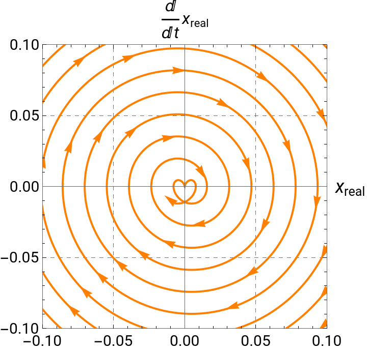
We are zooming the above plot to see the behaviour of our trajectories.
We have added arrows to our trajectories to understand how it evolves with time.
We have added arrows to our trajectories to understand how it evolves with time.
In the next section, we have solved the differential equation using the numerical method provided by Wolfram and compared it with the solutions reproduced by the renormalization approach .
In[]:=
s=NDSolve[{xr''[t]-2*m1*xr[t]*xi[t]*xr'[t]+m1*xi'[t]-m1*xi'[t]+m1*xi'[t]*+2*m2*xr'[t]*yr[t]*yi[t]-m2*xi'[t]+m2*xi'[t]*-m2*xi'[t]*+xr[t]0,xi''[t]-m1*xr'[t]+m1*xr'[t]*-m1*xr'[t]*-2*m1*xi'[t]*xr[t]*xi[t]+m2*xr'[t]-m2*xr'[t]*+m2*xr'[t]*+2*m2*xi'[t]*yr[t]*yi[t]+xi[t]0,yr''[t]+2*m1*xr[t]*xi[t]*yr'[t]-m1*yi'[t]+m1*yi'[t]*-m1*yi'[t]*-2*m2*yr'[t]*yr[t]*yi[t]+m2*yi'[t]-m2*yi'[t]*+m2*yi'[t]*+yr[t]0,yi''[t]+m1*yr'[t]-m1*yr'[t]*+m1*yr'[t]*+2*m1*yi'[t]*xr[t]*xi[t]-m2*yr'[t]+m2*yr'[t]*-m2*yr'[t]*-2*m2*yi'[t]*yr[t]*yi[t]+yi[t]0,xr[0]0.5,xi[0]0,yr[0]0.36,yi[0]0,xr'[0]==0,xi'[0]==0,yr'[0]==0,yi'[0]==0},{xr,xi,yr,yi},{t,0,1000}]
2
(xr[t])
2
(xi[t])
2
(yr[t])
2
(yi[t])
2
(xr[t])
2
(xi[t])
2
(yr[t])
2
(yi[t])
2
(xr[t])
2
(xi[t])
2
(yr[t])
2
(yi[t])
2
(xr[t])
2
(xi[t])
2
(yr[t])
2
(yi[t])
Out[]=
xrInterpolatingFunction,xiInterpolatingFunction,yrInterpolatingFunction,yiInterpolatingFunction


test10=Plot1=ParametricPlotEvaluate[{xr[t],xr'[t]}/.s],{t,0,320},(*Plottingoptions*);Zoom0=test10/.Line[rest_]{Arrowheads[Table[0.021,{i,0,1,.005}]],Arrow[BSplineCurve@rest]};
smalltest10=ParametricPlotEvaluate[{xr[t],xr'[t]}/.s],{t,0,320},;Zoom10=smalltest10/.Line[rest_]{Arrowheads[Table[0.05,{i,1,3,.002}]],Arrow[BSplineCurve@rest]}
Out[]=
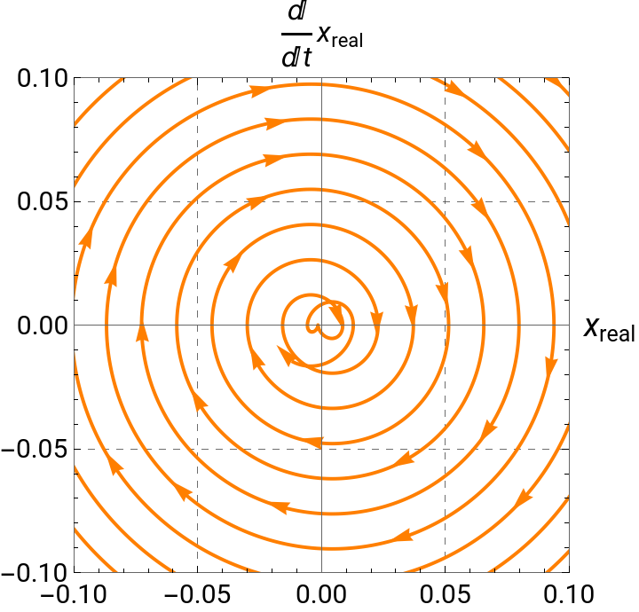
We are zooming the above plot to see the behaviour of our trajectories. We have added arrows to our trajectories to understand how it evolves with time.
The next plot is for m1 = m2, where we have plotted only for vs , since the vanishes for this specific condition of our parameters.
x
real
x'
real
x
img
test6=ParametricPlot0.5*Cos*Cos+*0.5*Sin*Sin-*0.5*Sin*Sin,-0.5*CosSin,{t,0,320},(*Plottingoptions*);Zoom2=test6/.Line[rest_]{Arrowheads[Table[0.05,{i,0,0.2,.1}]],Arrow[BSplineCurve@rest]}
2**(m1-m3)*(t-0)
2
1
4*-
2
1
2
(m1-m3)
4*(t-0)
3
1
4*-
2
1
2
(m1-m3)
m1
2*1
2**(m1-m3)*(t-0)
2
1
4*-
2
1
2
(m1-m3)
4*(t-0)
3
1
4*-
2
1
2
(m1-m3)
m3
2*1
2**(m1-m3)*(t-0)
2
1
4*-
2
1
2
(m1-m3)
4*(t-0)
3
1
4*-
2
1
2
(m1-m3)
2(m1-m3)(t-0)
2
1
-+4
2
(m1-m3)
2
1
4(t-0)
3
1
-+4
2
(m1-m3)
2
1
Out[]=
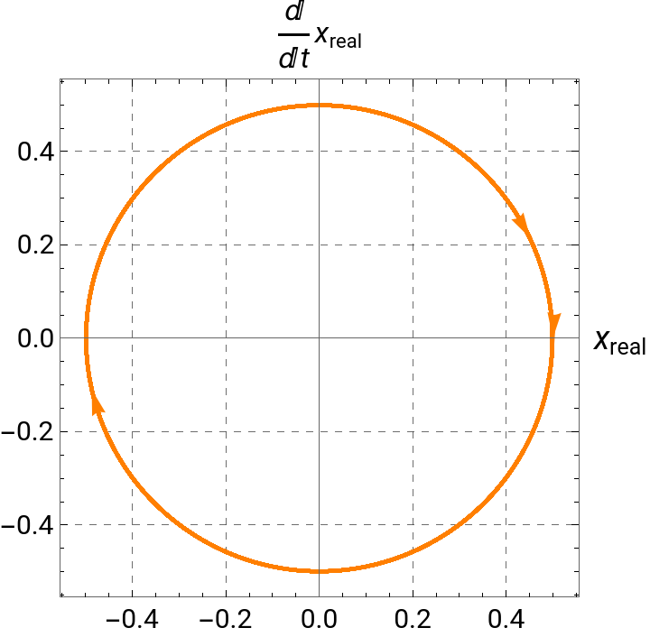
In the next section, we have solved the differential equation using the numerical method provided by Wolfram and compared it with the solutions reproduced by the renormalization approach .
We are zooming the above plot to see the behaviour of our trajectories. We have added arrows to our trajectories to understand how it evolves with time.
Generating the figure 3 plot from the paper
Generating the figure 3 plot from the paper
Here we demonstrate the PT phase transition
After the loop, the variable ‘ data’ contains pairs of the form : {m1, (fraction of complex eigenvalues to total number)} for each value of m1 = j . This can then be used for further analysis or plotting to investigate transitions in the spectral properties of the modified van der Pol oscillator .
Plotting the data that we got from the above analysis:
Generating the figure 4 plot from the paper
Generating the figure 4 plot from the paper
Initialize data lists for each fixed value of m1
First loop: Fixed m1 = 0.01, vary m2 from 0.001 to 0.1 in steps of 0.001
Second loop: Fixed m1 = 0.014, vary m2 from 0.001 to 0.1 in steps of 0.001
Third loop: Fixed m1 = 0.018, vary m2 from 0.001 to 0.1 in steps of 0.001
Plotting the data that we got from the above analysis:
Create a ListLinePlot to visualize the fraction of complex eigenvalues versus m1/m2
CITE THIS NOTEBOOK
CITE THIS NOTEBOOK
Renormalization Group Approach for Modified vdP Oscillator with Symmetric Non-Hermitian Interaction
by Biswajit Bhowmick, Rohit Mahendra Shinde & Bhabani Prasad Mandal
Wolfram Community, STAFF PICKS, March 11, 2025
https://community.wolfram.com/groups/-/m/t/3415513
by Biswajit Bhowmick, Rohit Mahendra Shinde & Bhabani Prasad Mandal
Wolfram Community, STAFF PICKS, March 11, 2025
https://community.wolfram.com/groups/-/m/t/3415513