Hepatitis B virus (HBV) and hepatitis delta virus (HDV) coinfection is considered the most severe form of chronic viral hepatitis. Drugs against HDV are under development, which serves as motivation to model the interplay between HBV and HDV under anti-HDV treatment. We first examine a simple differential equation model for studying the coinfection at the chronic stage, solving the model equations and performing the fitting. We offer an interactive user interface for experimenting with the model parameters. We then examine the HBV acute infection stage and model the dynamics of the cell-to-cell spread by cellular automata. We find out that a simple cellular automaton rule is able to capture a biphasic behavior in the HBV cell-to-cell spread of the infection. As future work, cellular automata can be extended to model more features in the dynamics of the HBV acute infection and study its multi-phases that have been observed.
Modeling the Coinfection of HBV and HDV
Modeling the Coinfection of HBV and HDV
The coinfection occurs at the chronic stage and a variety of differential equation models have been developed, as detailed in [1]. These are compartmental models that can also be analyzed with RobertNachbar/CompartmentalModeling that is available in the Wolfram Language Paclet Repository.
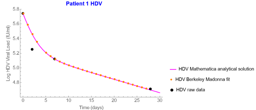
We present a simple differential equation model in which there is an equation for HDV and an equation for HBV, and the two equations are coupled. The variables are the HDV viral load and the HBV viral load. There are a few parameters in the model, as described in [1], which also provides a schematic diagram for the model. Such types of models arising in immunology, if simple enough, can be usually solved numerically with a specialized software package called Berkeley Madonna that can be found at http://berkeley-madonna.myshopify.com . However, the Wolfram Language can provide closed-form solutions to the model equations that Berkeley Madonna cannot. We show in the sequel that we can use Mathematica to perform the fitting as well, obtaining results that are highly similar to the ones obtained with Berkeley Madonna, with the advantage of having closed-form solutions to the model equations.
We present a simple differential equation model in which there is an equation for HDV and an equation for HBV, and the two equations are coupled. The variables are the HDV viral load and the HBV viral load. There are a few parameters in the model, as described in [1], which also provides a schematic diagram for the model. Such types of models arising in immunology, if simple enough, can be usually solved numerically with a specialized software package called Berkeley Madonna that can be found at http://berkeley-madonna.myshopify.com . However, the Wolfram Language can provide closed-form solutions to the model equations that Berkeley Madonna cannot. We show in the sequel that we can use Mathematica to perform the fitting as well, obtaining results that are highly similar to the ones obtained with Berkeley Madonna, with the advantage of having closed-form solutions to the model equations.
A simple viral dynamics model for studying the coinfection of HBV and HDV
A simple viral dynamics model for studying the coinfection of HBV and HDV
The two coupled differential equations that comprise the model are provided below, after the insertion of some clinical data. For simplicity, we only use a single patient. We then solve the model equations using the Wolfram Language, perform the fitting using NMinimize (the procedure below can serve for illustration), compare with the Berkeley Madonna fit, and provide an interactive user interface using Manipulate for experimenting with the model parameters.
[1] Initialization
(*performed in an initialization cell at the bottom*)
(*performed in an initialization cell at the bottom*)
[2] Initial clinical values and model parameters as tuned with the Berkeley Madonna specialized software
In[]:=
B0=30200;(*initialHBVclinicalvalueforpatient#1*)D0=550000;(*initialHDVclinicalvalueforpatient#1*)c=0.51;n=2.4;e=0.73;g=0.042;
[3] Clinical data for patient #1
In[]:=
p1hdv={{0,5.74},{2,5.25},{7,5.12},{28,4.71}};p1hbv={{0,4.47},{2,4.08},{7,4.42},{14,4.57}};
[4] Sample data for patient #1 obtained from the Berkeley Madonna HDV and HBV fitted graphs
In[]:=
p1hdvm={{0.1,5.73982},{1.1,5.5884},{2.1,5.4596},{3.1,5.35435},{5.1,5.20665},{6.1,5.15671},{7.1,5.11737},{8.1,5.08537},{9.1,5.05829},{10.1,5.03442},{11.1,5.01262},{12.1,4.99213},{13.1,4.97248},{14.1,4.95335},{15.1,4.93456},{16.1,4.91597},{17.1,4.89751},{18.1,4.87913},{19.1,4.8608},{20.1,4.84251},{21.1,4.82424},{22.1,4.80597},{23.1,4.78772},{24.1,4.76947},{25.1,4.75123},{26.1,4.73298},{27.1,4.71474}};p1hbvm={{0.1,4.44853},{1.1,4.2418},{2.1,4.06921},{3.1,3.97301},{5.1,4.06373},{6.1,4.17333},{7.1,4.28038},{8.1,4.37536},{9.1,4.45751},{10.1,4.52888},{11.1,4.59199},{12.1,4.64907},{13.1,4.70187},{14.1,4.7517},{15.1,4.79949},{16.1,4.84591},{17.1,4.89142},{18.1,4.93632},{19.1,4.98082},{20.1,5.02507},{21.1,5.06914},{22.1,5.11311},{23.1,5.15701},{24.1,5.20086},{25.1,5.24469},{26.1,5.2885},{27.1,5.33229}};
[5] HDV and HBV ODEs and their closed-form solution as derived by Mathematica
In[]:=
hdvode=d'[t]==(1-e)cD0Exp[-gt]-cd[t];hdvsol=DSolve[{hdvode,d[0]==D0},d[t],t]//Simplifyhdvode2=d0'[t]==(1-e0)cD0Exp[-g0t]-cd0[t];hdvsol2=DSolveValue[{hdvode2,d0[0]==D0},d0[t],t]hbvode=b'[t]==cB0n^-4D0^n(d[t]/.hdvsol[[1]])^-n-cb[t];hbvsol=DSolve[{hbvode,b[0]==B0},b[t],t]//Simplifyhbvsolb=3.426628649627561`*^-10-0.5125181449450894`+8.81332735115094`*^13+1.`Hypergeometric2F1[2.4`,3.7051282051282053`,4.705128205128205`,-0.41689373297002724`];
1
3/5
(367.`+153.`)
117t/250
4
n0
-0.5100000000000001`t
n0
550000.`
3/5
(367.`+153.`)
117t/250
3/5
(367.`+153.`)
117t/250
4
n0
n0
550000.`
2.04`t
3/5
((367.`+153.`))
-51t/100
117t/250
0.468`t
Out[]=
{{d[t]388173.+161827.}}
-0.51t
-0.042t
Out[]=
550000.-0.51-0.51e0+0.51e0+1.g0
-0.51t
(0.51-1.g0)t
(0.51-1.g0)t
-0.51+1.g0
Out[]=
b[t]29883.3+
-0.51t
617.863Hypergeometric2F1[2.4,3.70513,4.70513,-0.416894]
1.53t
3/5
(367.+153.)
-51t/100
-21t/500
0.468t
3/5
(367.+153.)
117t/250
[6] Parameter fitting and numerical solution using Mathematica
In[]:=
hdvodep=d'[t]==(1-e1)cD0Exp[-g1t]-cd[t];hbvodep=b'[t]==cB0n1^-4D0^n1(d[t])^-n1-cb[t];pfun=ParametricNDSolveValue[{hdvodep,d[0]==D0,hbvodep,b[0]==B0},{d,b},{t,0,28},{e1,g1,n1}];tvals={{0,2,7,28},{0,2,7,14}};data={{5.74,5.25,5.12,4.71},{4.47,4.08,4.42,4.57}};model1[ee_?NumericQ,gg_?NumericQ,nn_?NumericQ]:=Norm[Log10[MapThread[#1[#2]&,{pfun[ee,gg,nn],tvals}]]-data];fit=Last[NMinimize[{model1[e1,g1,n1],e1<1,g1>0.01},{e1,g1,n1}]]e11=e1/.fit;g11=g1/.fit;n11=n1/.fit;hdvodep1=d'[t]==(1-e11)cD0Exp[-g11t]-cd[t];hdvsol1=DSolve[{hdvodep1,d[0]==D0},d[t],t]//Simplify;hdvnum=NDSolve[{hdvodep1,d[0]==D0},d,{t,0,28}];hbvodep1=b'[t]==cB0n11^-4D0^n11(d[t]/.hdvsol1[[1]])^-n11-cb[t];hbvnum=NDSolve[{hbvodep1,b[0]==B0},b,{t,0,28}];
Out[]=
{e10.717713,g10.0454555,n12.21493}
[7] Plots of the above with parameter values selection option
In[]:=
plot1=Plot[Evaluate[Log[10,d[t]]/.hdvsol],{t,0,30},PlotLegendsPlaced[{"HDV Mathematica analytical solution"},{1,0.4}],PlotStyleMagenta,FrameLabel{"Time (days)","Log HDV Viral Load (IU/ml)"},PlotLabelStyle["Patient 1 HDV",Blue,Bold]];plot1a=Plot[Evaluate[Log[10,d[t]]/.hdvnum],{t,0,30},PlotLegendsPlaced[{"HDV Mathematica fitted solution"},{1,0.5}],PlotStyle{Green,Dashed}];plot2=ListPlot[{p1hdv},PlotStyle->Black,PlotMarkers{Automatic},PlotLegendsPlaced[{"HDV raw data"},{1,0.2}]];plot2a=ListPlot[{p1hdvm},PlotStyle->Orange,PlotLegendsPlaced[{"HDV Berkeley Madonna fit"},{1,0.3}]];plot4=Plot[Evaluate[Log[10,b[t]]/.hbvsol],{t,0,30},PlotStyle->Magenta,PlotLegendsPlaced[{"HBV Mathematica analytical solution"},{1,0.4}],FrameLabel{"Time (days)","Log HBV Viral Load (IU/ml)"},PlotLabelStyle["Patient 1 HBV",Blue,Bold]];plot4a=Plot[Evaluate[Log[10,b[t]]/.hbvnum],{t,0,30},PlotStyle->{Green,Dashed},PlotLegendsPlaced[{"HBV Mathematica fitted solution"},{1,0.5}]];plot5=ListPlot[{p1hbv},PlotStyle->Black,PlotLegendsPlaced[{"HBV raw data"},{1,0.2}]];plot5a=ListPlot[{p1hbvm},PlotStyle->Orange,PlotLegendsPlaced[{"HBV Berkeley Madonna fit"},{1,0.3}]];Show[plot1,plot2,plot2a]With[{sold=Simplify[hdvsol2]},Manipulate[LogPlot[sold,{t,0,30}],{{g0,0.042},0.01,0.1},{{e0,0.73},0,1},FrameLabel{"Time (days)","Viral Load (IU/ml)"},ControlPlacement->Right,SaveDefinitions->True]]Show[plot4,plot5,plot5a]With[{solb=Simplify[hbvsolb]},Manipulate[LogPlot[solb,{t,0,30}],{{n0,2.4},1,10},FrameLabel{"Time (days)","Viral Load (IU/ml)"},ControlPlacement->Right,SaveDefinitions->True]]
Out[]=
Initialization
Modeling the Acute Infection of HBV
Modeling the Acute Infection of HBV
The acute infection is occurring earlier than the chronic stage. For the acute infection of HBV, agent-based modeling has recently been developed in [2] in order to study the multi-phasic behavior that has been experimentally observed. With differential equation models, it is not trivial at all to capture this type of dynamics. Here we approach the modeling of the HBV acute infection by cellular automata. As a general reference for cellular automata, the reader is referred to the book “A New Kind of Science” by Stephen Wolfram. In immunology, one of the earliest works that utilize cellular automata is by Alan Perelson and coworkers described in https://link.springer.com/chapter/10.1007/978-3-642-76977-1_14 . The approach here provides a starting point for extending cellular automata to model acute viral hepatitis using the Wolfram Language.
We present a simple cellular automaton rule that demonstrates a biphasic behavior that can be captured in the governing dynamics. In the rule, we include three types of cells: non-infected cells, non-productive infected cells, and productive infected cells. We assume that before the start of our simulation, cell-free infection took place, and from here on there is cell-to-cell infection. Thus, in our initial condition there are infected cells in a variety of locations, and the rule controls the cell-to-cell spread from non-infected cells to non-productive infected cells to productive infected cells. By this simple rule, we are able to distinguish between two phases in the plot for the productive infected cells.
We present a simple cellular automaton rule that demonstrates a biphasic behavior that can be captured in the governing dynamics. In the rule, we include three types of cells: non-infected cells, non-productive infected cells, and productive infected cells. We assume that before the start of our simulation, cell-free infection took place, and from here on there is cell-to-cell infection. Thus, in our initial condition there are infected cells in a variety of locations, and the rule controls the cell-to-cell spread from non-infected cells to non-productive infected cells to productive infected cells. By this simple rule, we are able to distinguish between two phases in the plot for the productive infected cells.
A simple cellular automaton rule for modeling HBV acute infection
A simple cellular automaton rule for modeling HBV acute infection
The cellular automaton rule for simulating the spread of infection is provided below, after which we can run the simulation to a flexible number of steps and follow the spread at each step. Non-infected cells are denoted by 0, non-productive infected cells are denoted by 1, and productive infected cells are denoted by 2. In using RandomChoice with a combination of non-infected and infected cells, we assume that cell-free infection took place before the start of our simulation. Using Manipulate, we can keep track of the cell-to-cell spread as the number of steps increases. We then plot the time-dependent trajectory for each type of cell and are able to capture a biphasic behavior in the trajectory for the productive infected cells, as observed in Figures 4 and 6 of [2].
[1] Cellular automaton rule
[2] Initial condition and simulation of the acute infection
[3] Checks and a table representation
[4] Plots of the above showing a biphasic behavior
Concluding remarks
Concluding remarks
In this project, we present two simple hepatitis viral dynamics models and apply the Wolfram Language to solve the models and simulate the dynamics. We provide an interactive user interface that is friendly to use and illustrates the time-dependent behavior. We are modeling hepatitis viruses that are less researched at this time as compared to the well-studied HCV, namely HBV and HDV, at two different stages (chronic and acute) and two different modeling approaches (differential equations and cellular automata). The two simple models that are presented mainly serve for illustration purposes, capturing some of the basics of the underlying dynamics and providing ideas for further extensions.
In the case of the HBV acute infection, cellular automata are originally used for this problem and provide an interesting result. Even though the cellular automaton rule is very simple, it is able to capture a biphasic behavior in the spread of the infection. Interesting questions arise for further investigation, such as: to what extent is the cell-free infection playing an important role as compared to the cell-to-cell spread in HBV? Would it be more pronounced than in HCV? Would we be able to explain some of the more complex kinetic patterns with the different multi-phases that have been experimentally observed in chimeric mice with humanized livers [2], for discovering more about the properties of the virus?
At least some of these questions could be addressed by future extensions of the model. The simple rule does not account for the virus itself directly (the rule only considers non-infected cells, non-productive infected cells, and productive infected cells). Thus, the rule does not contain the clearance of the free virus, as well as other ingredients that are primarily suggested in the schematic diagram of Figure 2 in [2] such as the formulas for viral production, time interval between production cycle, and beyond. The rule is deterministic and does not contain any probabilistic considerations in it. Such ingredients and others can be incorporated to the cellular automaton simple rule in the future, for further studying the properties of the hepatitis B virus.
Keywords
Keywords
◼
HBV-HDV coinfection
◼
HBV acute infection
◼
Viral dynamics
◼
Cellular automata
Acknowledgment
Acknowledgment
I would like to thank my mentor Christopher Wolfram for his comprehensive help and insightful introduction to cellular automata, Bob Nachbar for his thorough feedback and suggestions on the compartmental modeling aspects, and Stephen Wolfram for encouraging me to expand the scope of my project beyond differential equation models. Work was performed in collaboration with Rami Zakh (Ben-Gurion University) and Harel Dahari (Loyola University Chicago).
References
References
◼
[1] R. Zakh, A. Churkin, W. Bietsch, M. Lachiany, S.J. Cotler, A. Ploss, H. Dahari, D. Barash (2021): A Mathematical Model for Early HBV and -HDV Kinetics during Anti-HDV Treatment, Mathematics Journal Special Issue on Mathematical and Computational Biology of Viruses at the Molecular or Cellular Levels, 9(24), 3323.
◼
[2] A. Hailegiorgis, Y. Ishida, N. Collier, M. Imamura, Z. Shi, V. Reinharz, M. Tsuge, D. Barash, N. Hiraga, H. Yokomichi, C. Tateno, J. Ozik, S.L. Uprichard, K. Chayama, H. Dahari (2023): Modeling Suggests that Virion Production Cycles within Individual Cells is Key to Understanding Acute Hepatitis B Virus Infection Kinetics, PLOS Computational Biology, In Press.
CITE THIS NOTEBOOK
CITE THIS NOTEBOOK
Viral dynamics modeling for Hepatitis B virus (HBV) and Hepatitis Delta virus (HDV)
by Danny Barash
Wolfram Community, STAFF PICKS, July 12, 2023
https://community.wolfram.com/groups/-/m/t/2958598
by Danny Barash
Wolfram Community, STAFF PICKS, July 12, 2023
https://community.wolfram.com/groups/-/m/t/2958598