The Wolfram Emerging Leaders Program: High School (WELP:HS) is a remote, semester-long program designed for exceptional graduates from the Wolfram High School Summer Research Program to continue to develop their skills. Students work in a small group over the course of a semester to do either a research-based project or a product development–based project under the guidance of expert mentors. Projects are centered around a topic at the intersection of the group’s interests.
Authors
Abstract
In this paper, we explore Wolfram Language implementations of multiple established computational methods for protein analysis, such as alpha complexes and Zernike moments. Existing methods for estimating a protein’s internal surface area, including the Voronoi method and the Occluded Surfaces algorithm, are computationally intensive and take a long time to run. To address this, we introduce a more efficient, novel Monte Carlo-based approach for estimating a protein’s internal surface area, which approximates these surfaces using randomized point distributions. A comparative analysis depicts that this method is highly accurate. This research contributes to the development of more efficient computational tools for protein analysis.
Alpha Complexes
Background
Background
Alpha complexes are a subset of Delaunay triangulations which are a robust mathematical framework to model molecular interactions and geometrical properties. This part of the essay looks at the implementation and visualisation of alpha complexes for a protein molecule using its atomic coordinates and Van der Waals radii.
Implementation
Implementation
We begin by representing the molecular structure of a protein using its SMILES string. Coordinates and Van der Waals radii for each atom are computed:
In[]:=
protein=Molecule["C(CCNC(=O)O)C[C@@H](C(=O)N)N"];coordinates=QuantityMagnitude[MoleculeValue[protein,"AtomCoordinates"],"Angstroms"];
In[]:=
vdwRadii=QuantityMagnitude[EntityValue[MoleculeValue[protein,"AtomList"]/.Atom[symbol_]:>Entity["Element",symbol],EntityProperty["Element","VanDerWaalsRadius"]],"Angstroms"];
The power distance is calculated which quantifies the squared difference between a point and a sphere:
In[]:=
powerDistance[x_,a_,r_]:=Norm[x-a]^2-r^2;
A function is defined which is used to check if two spheres overlap under an alpha parameter using both euclidean as well as power distance criteria to ensure appropriate inclusion:
In[]:=
alphaComplexOverlapQ[a_,b_,alpha_]:=Module[{dist2=Norm[coordinates[[a]]-coordinates[[b]]]^2},dist2<(vdwRadii[[a]]+vdwRadii[[b]])^2&&powerDistance[coordinates[[b]],coordinates[[a]],vdwRadii[[a]]+alpha]<dist2&&powerDistance[coordinates[[a]],coordinates[[b]],vdwRadii[[b]]+alpha]<dist2];
Now, alpha complexes are built by evaluation of pairwise overlaps among atoms. A modular approach is used to consider atomic subsets and an alpha parameter to construct facets of the alpha complex.
In[]:=
buildAlphaComplex[molA_,molB_,alpha_]:=Select[Flatten[Outer[List,molA,molB,1],1],alphaComplexOverlapQ[#[[1]],#[[2]],alpha]&];
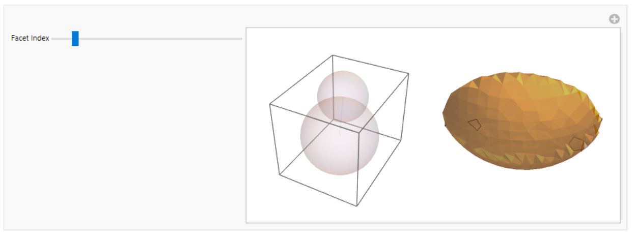
To visualize the overlap and relationships, functions to plot intersecting spheres and their corresponding regions are written:
In[]:=
plotIntersection[{a_,b_}]:=Module[{centerA=coordinates[[a]],centerB=coordinates[[b]],radiusA=vdwRadii[[a]],radiusB=vdwRadii[[b]]},Grid[{{Graphics3D[{Opacity[0.2],Sphere[centerA,radiusA],Sphere[centerB,radiusB],Blue,Line[{centerA,centerB}]}],RegionPlot3D[ImplicitRegion[(Norm[{x,y,z}-centerA]<=radiusA)&&(Norm[{x,y,z}-centerB]<=radiusB),{x,y,z}],PlotStyle->Opacity[0.5],Boxed->False,Axes->False,PlotRange->All]}}]];
The facets are now computed and are visualized:
In[]:=
splitPoint=Ceiling[Length[coordinates]/2];alphaComplexFacets=buildAlphaComplex[Range[splitPoint],Range[splitPoint+1,Length[coordinates]],0.1];
In[]:=
Manipulate[If[Length[alphaComplexFacets]>0,plotIntersection[alphaComplexFacets[[facetIndex]]],Graphics3D[Text["No facets available"]]],{{facetIndex,1,"Facet Index"},1,Length[alphaComplexFacets],1,Slider}]
A generalized approach is also worked out to simplify the alpha complex to any set of coordinates and radii:
In[]:=
buildAlphaComplex[coordinates_,radii_]:=Module[{pairs},pairs=Subsets[Range[Length[coordinates]],{2}];Select[pairs,EuclideanDistance[coordinates[[#[[1]]]],coordinates[[#[[2]]]]]<=(radii[[#[[1]]]]+radii[[#[[2]]]])&]];
In[]:=
alphaComplexFacets=buildAlphaComplex[coordinates,vdwRadii];
The facets and spheres are combined and graphically represented .
This overlays the Van der Waals spheres with lines representing alpha complex edges.
In[]:=
Graphics3D[Table[{Opacity[0.3],Sphere[coordinates[[i]],vdwRadii[[i]]]},{i,Length[coordinates]}]~Join~Table[{Red,Line[{coordinates[[f[[1]]]],coordinates[[f[[2]]]]}]},{f,alphaComplexFacets}],Boxed->False]
Out[]=

Analysis of Molecular Structure using Zernike Moments
Background
Background
Molecular shape is a fundamental aspect used to determine the physical and chemical properties of a molecule. Molecular structures can be better understood if quantified. Quantification allows researchers to explore how molecules interact with one another, how they bind to receptors, or how they might behave in specific environments. Computational tools play an important role by providing ways to measure, model, and compare molecular shapes with efficiency.
A powerful tool in computational chemistry is the use of Zernike moments which are mathematical descriptors that help us represent three dimensional shapes in a compact and rotationally invariant manner. Zernike moments can be used to reduce the complexity of molecular geometries in a manner such that the essential features that define their structure are preserved. This makes them a sought-after tool for applications like molecular docking, drug design, and structural comparisons across diverse chemical databases.
Spherical harmonics (𝑌(𝜃, 𝜙)) represent the angular variation of the molecular density distribution. Zernike moments use spherical harmonics as part of their basis functions to decompose and describe the 3D shape of a molecule in terms of radial and angular components.
Here’s a visualisation:
In[]:=
Plot3D[Abs[SphericalHarmonicY[2,1,theta,phi]],{theta,0,Pi},{phi,0,2Pi},ColorFunction->"SunsetColors",MeshFunctions->{#3&},PlotRange->All,AxesLabel->{"θ","φ","Amplitude"},PlotLabel->"Spherical Harmonics |Y2,1|"]
Out[]=

Zernike polynomials are a set of orthogonal polynomials defined on the unit disk, and they are represented in polar coordinates (𝜌,𝜃) where: 𝜌 is the radial distance (from the origin, 0 ≤ 𝜌 ≤ 1) and 𝜃 is the angular coordinate (from 0 to 2𝜋).
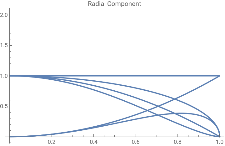
The radial component is useful in defining the shape and capturing the image information. It depends only on 𝜌 and determines how the polynomial varies with distance from the origin, independent of the angle.
The radial component is useful in defining the shape and capturing the image information. It depends only on 𝜌 and determines how the polynomial varies with distance from the origin, independent of the angle.
The radial component function for different values of 𝑛 and 𝑙 are plotted here:
In[]:=
radialComponent[n_,l_,r_]:=r^l (1-r^2)^((n-l)/2);radialPlot=Table[Plot[radialComponent[n,l,r],{r,0,1},PlotLabel->"Radial Component"],{n,0,3},{l,0,n,2}];Show[radialPlot]
Out[]=
Workflow
Workflow
The workflow of this project includes:
◼
Extraction of atomic positions and radii from a molecular structure.
◼
Computation of a Gaussian density function for the molecule.
◼
Definition and calculation of Zernike moments up to a specified order.
◼
Normalization of these moments and usage of the Canterakis norm as a shape descriptor.
◼
Calculation of geometric and statistical measures to provide additional context about the molecule’s spatial distribution.
Implementation of Code
Implementation of Code
Here, we extract the atomic coordinates and Van der Waals radii for all atoms in the molecule:
In[]:=
molecule=Molecule["C(CCNC(=O)O)C[C@@H](C(=O)N)N"];
In[]:=
MoleculePlot3D[molecule]
Out[]=

The density contribution of each atom is written as a Gaussian function that is centered on its position. The Gaussian’s width is determined by the atomic radius and the function depends on the spherical coordinates (𝑟, 𝜃, 𝜙).
The total molecular density is then computed by summing individual atomic densities:
Zernike moments are now calculated using radial and spherical harmonic components. Here, the radial component describes the radial variation of the molecule while the spherical harmonic component encodes angular variation. Then, Zernike moments are computed as integrals of the molecular density function over 3D space.
The Zernike moments are computed up to a specific order and are normalized so that they could be compared across molecules. This is done by calculating the Canterakis norm which summarizes the moments.
Zernike moments are computed up to a specific order, in this case 3:
The Zernike moments are normalized:
Visualizing the Zernike moments:
To further characterize the molecule's shape, we compute the radius of gyration which is the average distance of atoms from the center of mass. Statistical measures which include standard deviation, skewness, and kurtosis of atomic distances are also computed. The percentiles which are quantiles of distances from the center of mass are calculated as well.
Here’s a plot of the atom positions along with the the radius of gyration and distances from the center of mass.
Conclusion
Conclusion
The computational methods mentioned above provide a detailed approach to analyzing molecular shape using Wolfram Language. Zernike moments are used to describe the 3D structure of the molecule in a concise and rotationally invariant way which are suitable for comparing shapes across different molecules. The Canterakis norm simplifies the comparison by converting Zernike moments into a single-shape descriptor. Geometric and statistical measures are used to add more context to the spatial distribution of atoms within the molecule. Future work could extend these analyses by incorporating more complex molecular features, such as charge distribution or flexibility to deepen our understanding the behaviour of molecular structures.
Calculating Internal Surface Area
Background
Background
Internal Surface Area
Internal Surface Area
The internal surface area of a protein is the surfaces between atoms of the protein that are not exposed to the outside. In other words, solvents can’t get to these surfaces within the proteins.
Internal surface area “correlates well with their hydrophobicity derived from amino acid transfer experiments”, and is important when considering protein stability in drug design (Millet et al., 1987).
The goal is to establish a new, more performant method to calculate this internal surface area, and compare its accuracy and time-efficiency with an established method.
Established Methods
Established Methods
We establish the following two methods: Voronoi interface and occluded surface. Voronoi (Figure 1a) creates planar interfaces between atoms, while occluded surface (Figure 1b) creates spherical intersections. Both calculate the interface area between atoms. Both methods have been previously implemented and tested, so we use them as a baseline for accuracy and computational performance.
We then examine a novel and more performant method based on Monte-Carlo ideals to determine ideal parameters to compromise the least amount of accuracy for the greatest performance gains.
Methods
Methods
Voronoi Interface
Voronoi Interface
calculateVoronoiInterface creates a Voronoi mesh around the atom coordinates of a protein molecule and generates the net surface area of all shared faces in the Voronoi mesh. The red faces in Figure 1a are the shared faces (interface areas) that we use in this method.
In the calculateVoronoiInterface method, a protein molecule is taken as input. The atom coordinates are extracted as well as the list of atoms in the input molecule. These coordinates are used to generate a Voronoi diagram. VoronoiMesh creates the mesh where each cell is used to represent the space closest to an atom.
MeshPrimitive extracts the 3D cells from the Voronoi mesh. correspondingCells finds the Voronoi cell that corresponds to the atom and has matching coordinates. The surface area of the Voronoi cells are calculated and changed based on the bounding region area. checkForSamePolygon checks that the Voronoi cell polygons that are around the same position/area are recognized as the same.
In this implementation, the Voronoi method is incredibly ill-performant because of its reliance on geometry methods. In limited testing, it does correlate with the following methods; results, however, are of such a small sample size that this method cannot be properly used nor compared.
Occluded Surface Area
Occluded Surface Area
calculateOccludedSurfaceArea is a function that takes a protein molecule as input. The coordinates and Van der Waals radii are extracted for each atom.
pointsOnSphere generates surface points of a sphere that has a radius equal to the Van der Waals radii. These points can be used to determine which parts of the surface are occluded by the neighboring atoms. The perpendicular vectors (normals are generated for the surface points. intersectionPoint checks if the two spheres generated for the atoms intersect. All atom pairs are checked to see if they are within a certain distance and the occluded surface area is then calculated. Ray tracing is used to see the length of the occlusion. The total OSA is found by summing all the blocked portions of all the atoms.
A New Method
A New Method
Conceptualizing Monte-Carlo in Surface Area Calculations
Conceptualizing Monte-Carlo in Surface Area Calculations
Monte-Carlo
Monte-Carlo
Monte-Carlo methods are not specific to chemistry. The idea behind a Monte-Carlo program is to try a lot of things. One of the most commonly known Monte-Carlo programs is a method for estimating Pi:
First scatter a large number of random points on a 2x2 square:
Then count the number of points that are within a unit circle:
To confirm, we multiply the fraction of points inside the circle by 4 and get 3.1416, which is accurate to π (3.1415...) within four significant figures.
Monte-Carlo in Context
Monte-Carlo in Context
It’s possible to use a similar idea here, to find the interface area of a molecule. The interface area is, in approximation, the area of every surface inside a molecule that is equidistant from the closest molecules to that surface.
So suppose a three-dimensional grid of scattered points is constructed within the bounding box of a molecule. Then by counting the number of those points that are (approximately) equidistant from the closest molecules to each point, it would be possible to estimate the interface area of a molecule without using geometry tools - the greatest overhead in the Voronoi method - and at high speed, thanks to the relatively performant calculations required.
To start, we define a small number of atoms. In this case, those atoms are just random three-dimensional points:
To construct the grid, we generate a uniform scattering of points at a defined density. The density is important because small molecules should have smaller surface areas than large molecules. If the grid were to contain the same number of molecules every time, scale would no longer play a part in the calculations.
Instead of doing costly trigonometric calculations, we find the surfaces by giving each point an “attraction vector”. The attraction vector is the sum of all “attraction forces” exerted by each atom, where each atom is given gravitational pull. Then, surfaces that are equidistant between two atoms will find the gravitational forces canceling out, and their attraction vectors to be close to 0.
Looking at the resulting force field, it’s clear that the correct surfaces are being identified with the attraction vectors.
When finding the surfaces, we need to define cutoffs to isolate the correct points by vector magnitude. To ensure this works for all atom configurations, regardless of scale or quantity, the vector magnitudes should be taken as proportions of their range.
One problem, however, is that some attraction vectors - particularly those very close to a molecule - have enormously large magnitudes.
To remove outliers, define fences using the interquartile range:
The opacity in this field graph prove that the adjusted range more uniformly normalizes the magnitudes.
Threading the grid and the attraction vectors simply removes additional loops that may be need later on:
Now that a range has been defined, any outliers can be removed:
The remaining points have been adequately selected, as seen below.
Filtering the field to only select those at the edges is done here:
The interface area is quantified—the unit being dependent on the density, and therefore only the relative scale being relevant—by the number of points within the bounds of the filter:
Graphing the selected points shows that the approximation is relatively accurate.
Implementing Monte-Carlo as a Function
Implementing Monte-Carlo as a Function
To use the concepts established above, a function needs to be created with more general values.
Density is the only user-controlled value, as everything works in proportions and therefore shouldn’t change molecule-to-molecule:
Testing Monte-Carlo in Reference to Established Methods
Testing Monte-Carlo in Reference to Established Methods
One thing to note here is that the Voronoi method is both hard to use and computationally expensive, and so cannot be considered in this comparison. It is assuredly magnitudes slower than any of the methods tested in this section.
Selecting some molecules from the database API:
The first methods of comparison will be timing and results.
Because density is almost directly proportional to time, different levels of accuracy and speed can be defined:
The occluded surface algorithm is also examined:
Monte-Carlo Timing
Monte-Carlo Timing
Even the default parameters yield promising timing and relatively linear scaling:
The fast version begins to show some less-linear scaling but is also a magnitude faster:
And the accurate version is more adherent to the linear scaling but also around three to four times slower (still remaining, at worst, around a second):
Occluded-Surface Timing
Occluded-Surface Timing
Occluded-surface is significantly slower, notably, than Monte-Carlo:
Monte-Carlo Timings and Occluded-Surface Timings Comparison
Monte-Carlo Timings and Occluded-Surface Timings Comparison
Comparing the timings by test case and method will yield a more comprehendible overview, so the next step is to visualize that.
Clearly, the Monte-Carlo timings are consistently significantly lower than Occluded-Surface. In fact, the standard and fast methods appear to regularly be a magnitude smaller.
It is a little difficult, however, to gauge some of the more minute differences in this chart because the timings have such extreme differences.
Trying linearization by logarithms is one solution to this issue:
And it’s clear that there really is a magnitude of difference between Monte-Carlo and Occluded-Surface.
Results
Results
The results of Monte-Carlo and Occluded-Surface line up pretty linearly:
And though the fast version of Monte-Carlo is evidently less accurate (relative to Occluded-Surface), it is still mostly linear:
There are actually very few accuracy gains (relative to time loss) when examining the accurate version:
Head-to-Head
Head-to-Head
It’s also important to consider whether Monte-Carlo agrees with Occluded-Surface in head-to-head molecule comparisons.
Establishing a small set of comparison pairs:
And presenting the data:
Although a small sample set, Monte-Carlo does usually agree with Occluded-Surface.
Conclusions
Zernike Moments
Zernike Moments
The computational methods mentioned above provide a detailed approach to analyzing molecular shape using Wolfram Language. Zernike moments are used to describe the 3D structure of the molecule in a concise and rotationally invariant way which are suitable for comparing shapes across different molecules. The Canterakis norm simplifies the comparison by converting Zernike moments into a single-shape descriptor. Geometric and statistical measures are used to add more context to the spatial distribution of atoms within the molecule. Future work could extend these analyses by incorporating more complex molecular features, such as charge distribution or flexibility to deepen our understanding the behaviour of molecular structures.
Internal Surface Area
Internal Surface Area
Our novel computational method for approximating internal surface areas of proteins yields promising results with relative accuracy and significant performance benefits. Given applications of calculating buried residues - including drug retargeting - we hope these results may result in further advances in larger projects.
Acknowledgements
Over the course of the development of this paper, we received help from the team behind the Wolfram Emerging Leaders Program.
Thank you to Dr. Jason Sonnenberg for his unrelenting willingness to help us with anything we needed, from chemistry we were struggling with to opaque Wolfram documentation that we couldn’t quite grasp.
Thank you to the leadership team, including Rory Foulger and Eryn Gillam, as well as to everyone else at Wolfram who responded to our help posts, worked behind the scenes, and took interest in our project.
References
Cazals F, Proust F, Bahadur RP, Janin J. Revisiting the Voronoi description of protein-protein interfaces. Protein Sci. 2006 Sep;15(9):2082-92. doi: 10.1110/ps.062245906. PMID: 16943442; PMCID: PMC2242599.
Frederic M. Richards, The interpretation of protein structures: Total volume, group volume distributions and packing density, Journal of Molecular Biology, Volume 82, Issue 1, 1974, Pages 1-14, ISSN 0022-2836, https://doi.org/10.1016/0022-2836(74)90570-1.
Uttamkumar Samanta, Ranjit P. Bahadur, Pinak Chakrabarti, Quantifying the accessible surface area of protein residues in their local environment, Protein Engineering, Design and Selection, Volume 15, Issue 8, August 2002, Pages 659–667, https://doi.org/10.1093/protein/15.8.659
Susan Miller, Joël Janin, Arthur M. Lesk, Cyrus Chothia, Interior and surface of monomeric proteins, Journal of Molecular Biology, Volume 196, Issue 3, 1987, Pages 641-656, ISSN 0022-2836, https://doi.org/10.1016/0022-2836(87)90038-6.
Dmytro Guzenko, Stephen K. Burley, Jose M. Duarte, Real time structural search of the Protein Data Bank, PLOS ONE, 2020, https://doi.org/10.1371/journal.pone.0243985.
CITE THIS NOTEBOOK
CITE THIS NOTEBOOK
Established and novel methods for protein analysis in Wolfram Language
by Wolfram Education Programs
Wolfram Community, STAFF PICKS, February 4, 2025
https://community.wolfram.com/groups/-/m/t/3379964
by Wolfram Education Programs
Wolfram Community, STAFF PICKS, February 4, 2025
https://community.wolfram.com/groups/-/m/t/3379964