Previous posts looked at recovering density over 0..1 from moments in Wolfram language
1. analytically from an infinite series of moments, part 1
2. numerically from a finite set of exact moments, part 2
This post will look
3. numerically from a finite set of inexact moments.
Moments are inexact when they are:
- specified using floating point, incurring round-off error.
- estimated from a finite sample, incurring estimation error.
For inexact moments, even numerically stable procedure may give nonsensical results.
In[]:=
SF=StringForm;
Example
Example
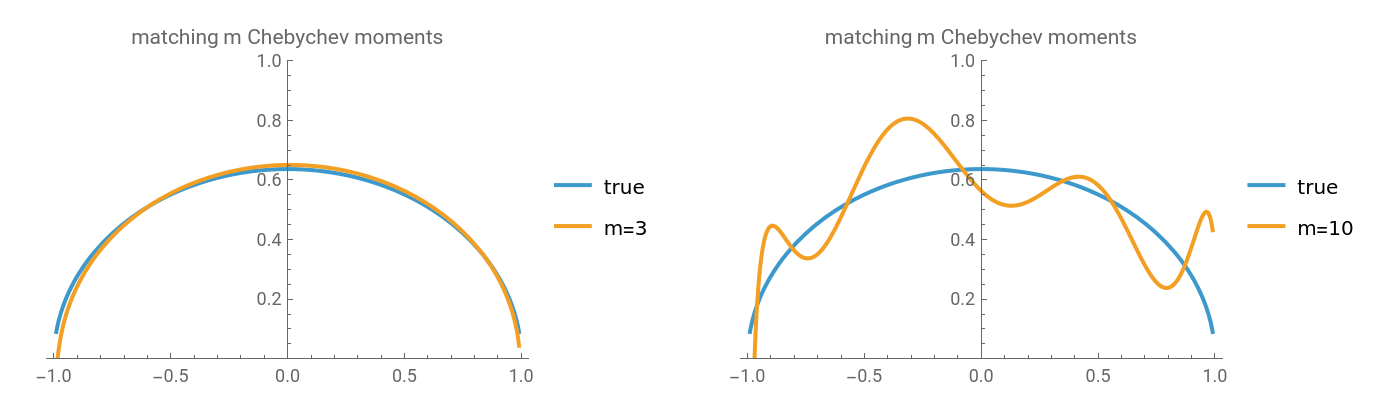
Consider estimating WignerSemicircle using Chebychev moment matching.
Matching first 3 moments is good. Matching first 10 moments is bad.
Matching first 3 moments is good. Matching first 10 moments is bad.
Out[]=
Quantify this by plotting Wasserstein-1 distance between target and moment-matched distribution, as a function of the number of moments matched
Out[]=
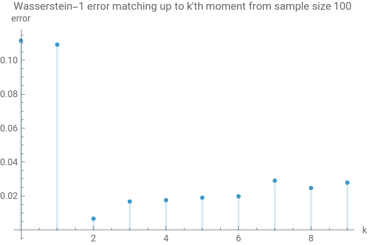
Error is the lowest for k=2, then it goes up again.
To see why, calculate the mean and variance of moment sample estimates:
To see why, calculate the mean and variance of moment sample estimates:
In[]:=
sampleMoment[k_]:=TransformedDistribution[ChebyshevT[k,x],xWignerSemicircleDistribution[1]];table=Table[#@sampleMoment[k]&/@{Mean,Variance},{k,kvals}];table=TableForm[table,TableHeadings->{{"E[]","Var[]"},SF["k=``",#]&/@kvals}]
m
k
m
k
Out[]//TableForm=
k=0 | k=1 | k=2 | k=3 | k=4 | k=5 | k=6 | k=7 | k=8 | k=9 | k=10 | |
E[ m k | 1 | 0 | - 1 2 | 0 | 0 | 0 | 0 | 0 | 0 | 0 | 0 |
Var[ m k | 0 | 1 4 | 1 4 | 1 2 | 1 2 | 1 2 | 1 2 | 1 2 | 1 2 | 1 2 | 1 2 |
Mean gives the true coefficient value, only 2 are non-zero.
Variance gives estimation error, it’s always non-zero
Approximation error bottoms out at zero for k>=2, estimation error grows monotonically.
Variance gives estimation error, it’s always non-zero
Approximation error bottoms out at zero for k>=2, estimation error grows monotonically.
Generalized moments
Generalized moments
To generalize, we project empirical density onto subspace spanned by orthogonal components , .., where is a polynomial of degree <= i.
- Fixing w(x) determines family
- coefficients of a least-square fit are linear combinations of raw moments.
Using w(x)=1 gives LegendreP family
Using PDF of ArcSin distribution gives ChebychevT
More generally, let w(x) be the PDF of Beta Distribution with parameters a, b.
- a=b=1 gives Uniform weight => LegendreP
- a=b=1/2 gives ArcSin weight => ChebychevT
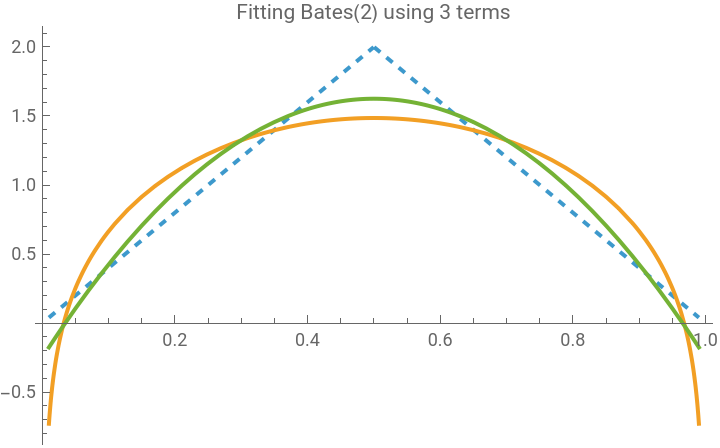
An example of using this to fit Bates(2) distribution:
w(x)(x)
p
0
w(x)(x)
p
m
p
i
- Fixing w(x) determines family
p
i
- coefficients of a least-square fit are linear combinations of raw moments.
Using w(x)=1 gives LegendreP family
Using PDF of ArcSin distribution gives ChebychevT
More generally, let w(x) be the PDF of Beta Distribution with parameters a, b.
- a=b=1 gives Uniform weight => LegendreP
- a=b=1/2 gives ArcSin weight => ChebychevT
An example of using this to fit Bates(2) distribution:
In[]:=
dot[a_,b_]:=Expectation[a,xb];fit[a_,b_,m_,target_]:=weight=BetaDistribution[a,b];p[k_]=JacobiP[k,b-1,a-1,2x-1];o[k_]=p[k]dot[o[k],target]o[k];m=3;{dist,distName}={BatesDistribution[2],"Bates(2)"};Plot@@{{PDF[dist,x],fit[1/2,1/2,m,dist],fit[1,1,m,dist]},{x,0.01,.99},PlotStyle->{Dashed,Automatic,Automatic},PlotLegends->{"target","Legendre, a=b=1","Chebychev, a=b=1/2"},PlotLabel->SF["Fitting `` using `` terms",distName,m]}
dot,weight
;(*orthonormalfamilyw.r.t.weight*);PDF[weight,x]2
p[k]
m
∑
k=0
Out[]=


Notes:
- Walter Gautschi proves this produces least squares fit in Section 3.2.1 (snippet) of his Orthogonal Polynomials book.
- The function could be negative, this can be avoided by damping coefficients, see A1 of https://arxiv.org/abs/2104.03461
- Walter Gautschi proves this produces least squares fit in Section 3.2.1 (snippet) of his Orthogonal Polynomials book.
- The function could be negative, this can be avoided by damping coefficients, see A1 of https://arxiv.org/abs/2104.03461
Expectation[a,xb] is known as the “generalized moment”
Because of orthonormality, these expectations are are coefficients of the least-squares fit
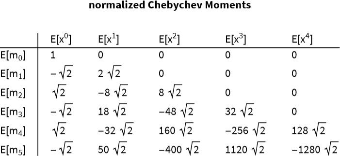
We can express k’th generalized moment as a linear combinations of first k raw moments using CoefficientList
Because of orthonormality, these expectations are are coefficients of the least-squares fit
We can express k’th generalized moment as a linear combinations of first k raw moments using CoefficientList
Out[]=
Out[]=
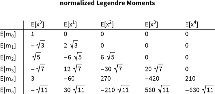
Parseval’s theorem to ensure fast decay
Parseval’s theorem to ensure fast decay
We’d like to pick a basis such that coefficients in that basis decay quickly.This requires that the series of coefficients is finite.Parseval’s theorem tells us that Fourier-transform is unitary.In our case, it connects the sum of squared coefficients to the integral of squared density.For coefficient decay, it is sufficient to pick weight such that is square-integrable.We verify Parseval connection by computing integral of squared density and checking that it’s equal to the sum of squared coefficients in Chebychev basis.1. Compute integral of squared density, divided by Chebychev weight
density
weight
In[]:=
a=1/2;b=1/2;weight=BetaDistribution[a,b];target=UniformDistribution[];integral=Integrate@@PDF[weight,x],{x,0,1}
2
PDF[target,x]
Out[]=
2
π
8
2. Sum of squared coefficients in orthonormal Chebychev basis
In[]:=
p[k_]=JacobiP[k,b-1,a-1,2x-1];norm2[k_]=dot,weight;(*originalslowversion*)norm2[k_]:=If[k==0,1,(2^(a+b-1)*Gamma[k+a]*Gamma[k+b])/((2*k+a+b-1)*k!*Gamma[k+a+b-1])/Beta[b,a]];o[k_]=p[k],{k,0,∞}]
2
p[k]
norm2[k]
;coef[k_]=Expectation[o[k],xtarget];Sum[2
coef[k]
Out[]=
2
π
8
To speed-up computation of orthonormal basis, I hard-coded squared norm formula from https://mathworld.wolfram.com/JacobiPolynomial.html, formula (10)
Summary
Summary
- Use fit(1/2,1/2, 5..) above to fit density over 0..1 using first 5 Chebychev moments- Use fit(1,1, 5..) above to fit density over 0..1 using first 5 Legendre moments- To ensure fast coefficient decay, pick parameters such that target/ is square integrable. For instance - fit(1/w, 1, ...) matches divergence at 0 - fit(1,1/w,...) matches ) divergence at 1
weight
w
Uniform
(1-
w
Uniform
CITE THIS NOTEBOOK
CITE THIS NOTEBOOK
Hausdorff moment problem: part 3, statistical efficiency
by Yaroslav Bulatov
Wolfram Community, STAFF PICKS, July 9, 2025
https://community.wolfram.com/groups/-/m/t/3497414
by Yaroslav Bulatov
Wolfram Community, STAFF PICKS, July 9, 2025
https://community.wolfram.com/groups/-/m/t/3497414