ABSTRACT (original article): Self-interacting random walks (SIRWs) show long-range memory effects that result from the interaction of the random walker at time with the territory already visited at earlier times . This class of non-Markovian random walks has applications in contexts as diverse as foraging theory, the behaviour of living cells, and even machine learning. Despite this importance and numerous theoretical efforts, the propagator, which is the distribution of the walker’s position and arguably the most fundamental quantity to characterize the process, has so far remained out of reach for all but a single class of SIRW. Here we fill this gap and provide an exact and explicit expression for the propagator of two important classes of SIRWs, namely, the once-reinforced random walk and the polynomially self-repelling walk. These results give access to key observables, such as the diffusion coefficient, which so far had not been determined. We also uncover an inherently non-Markovian mechanism that tends to drive the walker away from its starting point. CITATION (original article): Julien Brémont, Olivier Bénichou, Raphaël Voituriez (2024), Exact propagators of one-dimensional self-interacting random walks, arXiv:2404.15853. https://doi.org/10.48550/arXiv.2404.15853
t
t'<t
π quantities
π quantities
Here we prove the exactness of the functional equation approach.
Exact expression of the π quantities in the symmetric case
Exact expression of the π quantities in the symmetric case
In[]:=
Clear[thcoef,numcoef];Γ=3;u=;L=30;fpp[k_]:=(1+u)(Sinh[(k+1)μ]+Sinh[(k-3)μ]+2uSinh[(k-1)μ])((Sinh[kμ]+uSinh[(k-2)μ]));fpm[k_]:=(1+u)(Sinh[(k+1)μ]+Sinh[(k-3)μ]+2uSinh[(k-1)μ])((1-u)Sinh[μ])piexact[k_]:=NProduct[fpp[j],{j,1,L-k}]Productfpp[L+1-j]+fpm[L+1-j],{j,1,k};piexact[k_]:=NProduct[fpp[j],{j,1,L-k}]Productfpp[l+(L-k)+1]+fpm[l+(L-k)+1],{l,0,k-1};μ=;num=firstindex[L]//Simplify;numcoef=Table[SeriesCoefficient[num,{x,0,k}],{k,1,L-1}];thcoef=Table[pi[k],{k,1,L-1}];funceq=Table[piexact[k],{k,1,L-1}];plot=ListPlot[{numcoef,thcoef,funceq},PlotLegends->{"Numerical","Theory (diffusive limit)","Functional eq"},AxesLabel->{"k","π_(k,l)"},PlotMarkers->"OpenMarkers",PlotRange->All](*Export[StringTemplate["Nextcloud/These/Data/satw/Figures/exact-pik-L``-gamma-``-μ-``.pdf"][L,Γ,μ],plot];*)
1-Γ
1+Γ
2
u
2
u
Sinh[(k-j)μ]
Sinh[(k+1-j)μ]
Sinh[(L-k)μ]
Sinh[(k+1-j)μ]
Sinh[lμ]
Sinh[(l+1)μ]
Sinh[(L-k)μ]
Sinh[(l+1)μ]
20
L
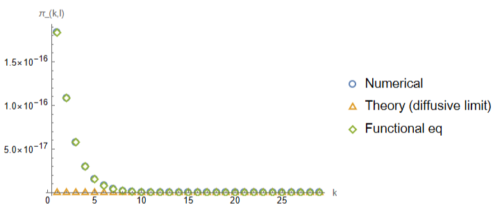
Exactcomputationoftheπk,L-katμ=0forSATW
Exactcomputationoftheatμ=0forSATW
π
k,L-k
In[]:=
id=IdentityMatrix[2];T={{0,1},{1,0}};X={{x,0},{0,1}};G[k_]:=IdentityMatrix[2]+T;glist[L_]:=Table[G[k].X,{k,1,L}];M[L_]:=Tr[Apply[Dot,Dot@@@Partition[glist[L],UpTo[10]]]]//Simplify;fullm[L_]:=Apply[Dot,Dot@@@Partition[glist[L],UpTo[10]]]//Simplifyfullm[3]+//MatrixFormfullm[7]+//MatrixForm
Γ
-1+k+Γ
31
O[x]
31
O[x]
Out[]//MatrixForm=
Γx 2+Γ 2Γ 2 x 2+Γ 3 x 31 O[x] | 1+ 2Γx 2+Γ Γ 2 x 2+Γ 31 O[x] |
Γx 2+Γ 2Γ 2 x 2+Γ 3 x 31 O[x] | 1+ 2Γx 2+Γ Γ 2 x 2+Γ 31 O[x] |

Click on the matrix above for higher resolution.
Notice how the ratio of one power k of x on one row from the first column to the second column is ALWAYS equal to . This is the key.
(k)
L-k
Propagator (computing the double sinh integral)
Propagator (computing the double sinh integral)
Computations and contiguous relations
Computations and contiguous relations
Below are the relevant hypergeometric functions entering in the calculations
In[]:=
fp:=Hypergeometric2F11+ϕ,,,;fbmfcm:=Hypergeometric2F1ϕ,,,;f:=Hypergeometric2F1ϕ,,,;
1-ϕ
2
3(ϕ+1)
2
-2β
E
-1-ϕ
2
3ϕ+1
2
-2β
E
1-ϕ
2
3(ϕ+1)
2
-2β
E
The formulae below are exact and have been checked. “contig” refers to the fact that we used a contiguous hypergeometric relation to simplify the expressions.
In[]:=
ψ1:=Beta,ϕfbmfcm;ψ2:=Beta,ϕf;ψ1contig:=Beta,ϕψ2contig:=Beta,ϕ;η1:=Beta,ϕfp;η1contig:=Beta,ϕCsch[β](1+3ϕ)Hypergeometric2F1(-1-ϕ),ϕ,(1+3ϕ),-(1+ϕ)Hypergeometric2F1,ϕ,,;η:=(η1(2Cosh[u]-Coth[β]Sinh[u])+Sinh[u](ψ1+ψ2));ηcontig1:=(η1contig(2Cosh[u]-Coth[β]Sinh[u])+Sinh[u](ψ1+ψ2));ηcontig2:=(η1(2Cosh[u]-Coth[β]Sinh[u])+Sinh[u](ψ1+ψ2contig));ηcontig3:=(η1(2Cosh[u]-Coth[β]Sinh[u])+Sinh[u](ψ1contig+ψ2));
1+ϕ
2
-βϕ
E
2
ϕ+1
Sinh[β]
1+ϕ
2
1+ϕ
1+3ϕ
-βϕ
E
2
ϕ+1
Sinh[β]
1+ϕ
2
-βϕ
E
2
ϕ+1
Sinh[β]
f+fϕ+4fpϕSinh[β]
-β
1+3ϕ
1+ϕ
2
1+ϕ
1+3ϕ
-βϕ
E
2
ϕ+1
Sinh[β]
fbmfcm+2(-1+)fpϕ+3fbmfcmϕ
-2β
1+ϕ
1+ϕ
2
2ϕ
1+3ϕ
-β(ϕ+1)
E
ϕ
Sinh[β]
1+ϕ
2
2ϕ
1+3ϕ
-β(ϕ+1)
E
ϕ
Sinh[β]
1
4ϕ
β
1
2
1
2
-2β
1-ϕ
2
3(1+ϕ)
2
-2β
ϕ
Sinh[β]
ϕ
Sinh[β]
ϕ
Sinh[β]
ϕ
Sinh[β]
In[]:=
Clear[ϕ];(*FullSimplify[ηcontig1]*)FullSimplify[ηcontig2](*FullSimplify[ηcontig3]*)
Out[]=
1
1+3ϕ
-β(3+2ϕ)
1+ϕ
2
β(3+ϕ)
1
2
1
2
-2β
β(2+ϕ)
1-ϕ
2
3(1+ϕ)
2
-2β
β
In[]:=
FullSimplify[ηcontig1]FullSimplify[ηcontig2]FullSimplify[ηcontig3]
Out[]=
1
2(1+3ϕ)
-βϕ
1+ϕ
2
1
2
1
2
-2β
1-ϕ
2
3(1+ϕ)
2
-2β
Out[]=
-β(1+ϕ)
1+ϕ
2
1
2
1
2
-2β
1-ϕ
2
3(1+ϕ)
2
-2β
Out[]=
1
1+3ϕ
-β(1+ϕ)
1+ϕ
2
β
1-ϕ
2
3(1+ϕ)
2
-2β
1-ϕ
2
3(1+ϕ)
2
-2β
In[]:=
Clear[ϕ];ϕ=4;Integrate,{α,0,∞},Assumptions->{u>0,β>0,ϕ>0}Integrate,{α,0,∞},Assumptions->{u>0,β>0,ϕ>0}ηfromint=(%%+%)//FullSimplify
ϕ
Sinh[α]
2ϕ+1
Sinh[α+β]
Sinh[α+u]
Sinh[α]
ϕ
Sinh[α]
2ϕ+1
Sinh[α+β]
Sinh[β-u]
Sinh[β]
ϕ
Sinh[β]
Check all relations
Contiguous relations
Contiguous relations
Check that indeed this relation holds
The following is thus the value of 2F1(a+1,b,c,z)
To replace f:
To replace fbmfcm:
Below is valid only for odd ϕ, because it is simpler to check.
Propagator in real space
Propagator in real space
Position of the bump (taking only two of the terms in the sum)
Diffusion coefficient
Diffusion coefficient
Asymmetric case
Asymmetric case
Computations
Computations
Then for η1
The weird Pochhammer formula that makes a lot of things simpler
Plots
Plots
Non-monotonicity
Non-monotonicity
Numerically : when are there bumps ?
Regularity
Regularity
Discontinuities
Discontinuities
Derivative
Derivative
CITE THIS NOTEBOOK
CITE THIS NOTEBOOK
Exact propagators of one-dimensional self-interacting random walks
by Julien Brémont, Olivier Bénichou and Raphaël Voituriez
Wolfram Community, STAFF PICKS, May 8, 2024
https://community.wolfram.com/groups/-/m/t/3172230
by Julien Brémont, Olivier Bénichou and Raphaël Voituriez
Wolfram Community, STAFF PICKS, May 8, 2024
https://community.wolfram.com/groups/-/m/t/3172230