We propose a systematic determination of all azeotropes for the following quaternary mixture composed of Methanol, Benzene, i-Propanol and n-Propanol at 1 atm using the Wilson model. Methanol, Benzene, i-Propanol and n-Propanol: are components 1 through 4 in the code below.
This problem was first treated by Fidkowski, Malone and Doherty (Ref.1) and their results are reproduced below:Finally, this problem was also solved by the late Prof. Floudas and co-workers using GAMS: see Chapter14 at: http://titan.princeton.edu/TestProblems/We benchmark our results, summarized in the Table below, against data generated by a Matlab bifurcation code written by several people at the CHE department of MIT including the late Prof. Swan.

Results of the bifurcation analysis:
This system has 3 binary azeotropes
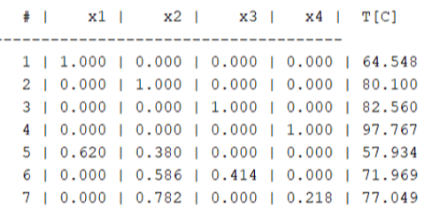
Bifurcation Diagram
Bifurcation Diagram
Doherty’s Homotopy Method (see Ref. 1)
ClearAll["Global`*"];
Constants
Ptot=760.0;(*totalpressure*)Rcal=1.9872041;(*universalgasconstant*)
components={"Methanol","Benzene","i-Propanol","n-Propanol"};abbrev={"Meth","Ben","i-ol","n-ol"};
Antoine Equation
In[]:=
antoineParams={{8.08097,1582.27,239.726},{6.87987,1196.76,219.161},{8.87829,2010.33,252.636},{8.37895,1788.02,227.438}};antoine[T_]:=Module[{Tc},Tc=T-273.15;10^(antoineParams[[All,1]]-antoineParams[[All,2]]/(antoineParams[[All,3]]+Tc))];
Wilson Model
V={38.8196,94.0952,79.6109,77.8926};AWilson={{0,1734.42,-38.4124,150.206},{183.038,0,392.702,312.162},{176.319,813.92,0,818.329},{-33.8819,996.275,-481.059,0}};lambdaWilson[T_]:=Table[If[i==j,1.0,(V[[j]]/V[[i]])*Exp[-AWilson[[i,j]]/(Rcal*T)]],{i,4},{j,4}];wilsonGamma[x_,T_]:=Module[{lam,S,lng},lam=lambdaWilson[T];S=lam.x;lng=Table[-Log[S[[k]]]+1-Sum[x[[i]]*lam[[i,k]]/S[[i]],{i,4}],{k,4}];Exp[lng]];
Pure components boiling temperatures
findTbp[i_]:=T/.FindRoot[antoine[T][[i]]-Ptot==0,{T,330}];Tbps=Table[findTbp[i],{i,4}];TbpsC=Tbps-273.15;
In[]:=
TbpsC
Out[]=
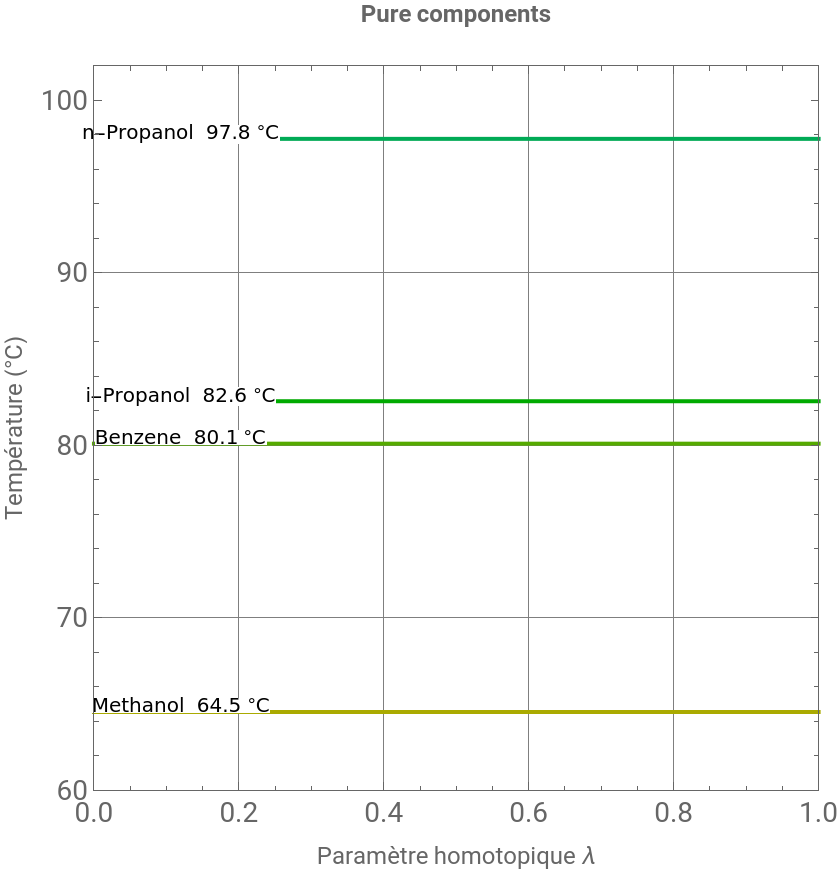
{64.5475,80.0996,82.56,97.7667}
Homotopy Equations
doherty[v_,la_]:=Module[{x3,x,T,psat,gam,K,f},x3=v[[1;;3]];x4=Max[1-Total[x3],10^-12];x=Join[x3,{x4}];x=x/Total[x];T=v[[4]];If[T<300||T>430,Return[ConstantArray[10^6,4]]];psat=antoine[T];gam=wilsonGamma[x,T];(*Correctthermodynamichomotopy*)K=(gam^la)*psat/Ptot;f=ConstantArray[0,4];Do[f[[i]]=x[[i]]*(K[[i]]-1),{i,3}];f[[4]]=K.x-1;f];
Initial guesses
initialGuesses={{0.62,0.38,0.000,330.},{0.000,0.586,0.414,345.0},{0.000,0.782,0.000,350.7}};
Azeotropes
azeotropes={};Do[sol=Quiet@FindRoot[doherty[{x1,x2,x3,T},1]=={0,0,0,0},{{x1,ig[[1]]},{x2,ig[[2]]},{x3,ig[[3]]},{T,ig[[4]]}},MaxIterations->500];xs={x1,x2,x3}/.sol;x4=Max[1-Total[xs],0];xx=Join[xs,{x4}];xx=xx/Total[xx];temp=T/.sol;If[Max[xx]<0.99,AppendTo[azeotropes,<|"x"->xx,"T"->temp-273.15,"v"->({x1,x2,x3,T}/.sol)|>]],{ig,initialGuesses}];azeotropes=DeleteDuplicates[azeotropes,Norm[#1["x"]-#2["x"]]<10^-3&];
Continuation
branches={};lambdaValues=N@Join[Range[0,0.8,0.02],Range[0.8,0.95,0.005],Range[0.95,1,0.001]];Do[v=az["v"];curve={};Do[sol=Quiet@FindRoot[doherty[{x1,x2,x3,T},la]=={0,0,0,0},{{x1,v[[1]]},{x2,v[[2]]},{x3,v[[3]]},{T,v[[4]]}},MaxIterations->300];v=({x1,x2,x3,T}/.sol);AppendTo[curve,{la,v[[4]]-273.15}],{la,Reverse@lambdaValues}];active=Flatten@Position[az["x"],_?(#>0.04&)];AppendTo[branches,<|"curve"->curve,"active"->active,"n"->Length[active],"T1"->az["T"]|>],{az,azeotropes}];
Colors
pureColors=Table[Darker@Hue[i/12],{i,2,5}];branchColors=Table[Darker@Hue[i/12],{i,2,4}];
Pure lines
pureLines=Table[{pureColors[[k]],Thick,Line[{{0,TbpsC[[k]]},{1,TbpsC[[k]]}}]},{k,4}];
Branch graphics
branchGraphics=Table[Module[{curve,col,style,n},curve=br["curve"];n=br["n"];col=branchColors[[Mod[i-1,Length[branchColors]]+1]];style=Which[n==2,Directive[col,Dashed,Thick],n==3,Directive[col,Dashed,Thick],n>=4,Directive[col,Dashed,Thick]];{style,Line[curve]}],{i,Length[branches]},{br,{branches[[i]]}}];
Pure component labels
pureLabels=Table[Text[Style[components[[k]]<>" "<>ToString@NumberForm[TbpsC[[k]],{4,1}]<>" °C",10,Black,Background->White],{0.12,TbpsC[[k]]+.35}],{k,4}];
Pure components lines
p=Show[Graphics[{pureLines,pureLabels}],Frame->True,FrameLabel->{Style["Paramètre homotopique λ",12],Style["Température (°C)",12]},LabelStyle->Directive[14],PlotRange->{{0.0,1.},{60,102}},GridLines->Automatic,ImageSize->420,AspectRatio->1,PlotLabel->Style["Pure components\n",12,Bold]]
Out[]=
References
References
[1] Z.T. Fidkowski, M.F. Malone, M.F. Doherty, Computing azeotropes in multicomponent mixtures, Computers & Chemical Engineering, Volume 17, Issue 12, 1993, Pages 1141-1155, https://doi.org/10.1016/0098-1354(93)80095-5
CITE THIS NOTEBOOK
CITE THIS NOTEBOOK
Systematic determination of the azeotropes of a quaternary system by bifurcation
by Samar Jebali, Oumaima ben saad, Ons Zarraa, Eya kefi, Yassmine ben hamouda, Housam Binous and Ahmed Bellagi
Wolfram Community, STAFF PICKS, May 25, 2026
https://community.wolfram.com/groups/-/m/t/3721533
by Samar Jebali, Oumaima ben saad, Ons Zarraa, Eya kefi, Yassmine ben hamouda, Housam Binous and Ahmed Bellagi
Wolfram Community, STAFF PICKS, May 25, 2026
https://community.wolfram.com/groups/-/m/t/3721533