This book provides a concise and practical introduction to quantum computing, emphasizing an interactive, hands-on approach. It introduces and explores the essential concepts, principles, and foundational quantum algorithms through guided modeling and simulation exercises. Each topic is developed computationally, allowing readers to build both intuition and technical proficiency by directly engaging with the computational mechanics of quantum systems. The approach taken here is computation first, meaning that understanding arises through the act of calculation, echoing David Mermin’s well-known slogan, “shut up and calculate.”
Full book: https://wolfr.am/QC-Book
Community post of part 1: https://community.wolfram.com/groups/-/m/t/3587974
Community post of part 1: https://community.wolfram.com/groups/-/m/t/3587974
Who is this book for? It is written for anyone curious about learning quantum computation through the lens of discrete vector spaces, seasoned with a delightful touch of quantum computing. I have deliberately avoided delving into the nitty-gritty of mathematical formalism. Instead, my focus is on computation itself, on doing the work, even when the underlying mathematics is complex and hidden behind the scenes. As I mentioned in the abstract, I believe one of the most important steps in learning quantum theory (an abstract and often intimidating subject at first encounter) is to learn by doing the computations.
The environment you will be working in is a Mathematica notebook. Every Mathematica notebook is organized into cells, each marked by a small bracket along the right edge of the window. A cell can contain text, visualizations, data, input code, or nearly anything else that can be expressed in computational form. In essence, it is a flexible workspace where ideas, mathematics, and computation come together seamlessly.
Many of the calculations in this book will be carried out using the Wolfram Quantum Framework. This framework is distributed as a paclet, meaning it is a collection of specialized functions. Once installed, these functions and their documentation pages become integrated into Mathematica, just like its native built-in functions. Do not get intimated by code. Even if it looks complicated, for many parts you can ignore the code and focus on the outcome.
If any question, please reach out to quantum@wolfram.com
Table of Contents (Part 2)
Deutsch-Jozsa Algorithm
We will discuss the Deutsch-Jozsa algorithm. It decides whether a promised function on n-bit inputs is constant or balanced using a single oracle call. The Deutsch-Jozsa circuit is designed in a way that if the function is constant, all amplitude concentrates on the all-zeros output; if balanced, that outcome vanishes and some nonzero string appears. A bit-flip oracle and a phase oracle are equivalent here because initializing the target in the minus state turns the bit flip into an input-dependent phase.
Key Concepts
Key Concepts
◼
Boolean function
◼
Constant Boolean function
◼
Balanced Boolean function
◼
Deutsch-Jozsa
Statement of the Deutsch-Jozsa Problem
Statement of the Deutsch-Jozsa Problem
You’re given black-box access to a Boolean function, , with the promise that is either constant, i.e. is the same for every (either all 0s or all 1s), or balanced, i.e, for exactly half of all inputs and for the other half.
f
f
f(x)
x
f(x)=0
f(x)=1
Let’s consider Xor in 3 variables, as a specific case, which is a balanced function. Keep in mind that you have a black-box access to it, and being told that it is either constant or balanced.
Count the number of False and True outputs over all 8 inputs for the 3-bit XOR (parity) function:
In[]:=
Counts@BooleanTable[Xor[x,y,z],{x,y,z}]
Out[]=
True4,False4
Let’s adopt a deterministic (always correct) classical algorithm. You query inputs one by one, observing . If you ever see both outputs 0 and 1, you can confidently say “balanced.” If all outputs seen so far are identical, you still don’t know: the function might be truly constant, or it might be balanced but you’ve only hit inputs from the “same half” so far. Therefore, any deterministic classical algorithm that is always correct needs, in the worst case, +1 queries (that’s exponential in .)
f(x)
n-1
2
n
Consider Xor in 3 variables as a specific example (). An adversary can keep you uncertain for a long time. For example, the inputs order can be like this:
n=3
In[]:=
allInputs=SortBy[Tuples[{True,False},3],Apply[Xor]]
Out[]=
{{False,False,False},{False,True,True},{True,False,True},{True,True,False},{False,False,True},{False,True,False},{True,False,False},{True,True,True}}
The outcome of queries on the list of inputs:
f
In[]:=
Xor@@@allInputs
Out[]=
{False,False,False,False,True,True,True,True}
Up to the fourth query, all outcomes are identical, so you cannot decide yet. The fifth query produces a different outcome, confirming the function is balanced. Let’s walk through the procedure step by step.
In[]:=
classicalDJ[Xor,allInputs]
The result of second query is the same as previous one, so still cannot determined if the function is balanced or constant.
The result of third query is the same as previous one, so still cannot determined if the function is balanced or constant.
The result of fourth query is the same as previous one, so still cannot determined if the function is balanced or constant.
After 5 queries, it is determined that the function is balanced
Now consider a different input ordering, for example, swap the 3rd and 5th entries from the previous list.
In[]:=
{allInputs[[3]],allInputs[[5]]}={allInputs[[5]],allInputs[[3]]};Xor@@@allInputs
Out[]=
{False,False,True,False,False,True,True,True}
This time, after the third query, you can conclude the function is balanced. Let’s walk through the steps.
In[]:=
classicalDJ[Xor,allInputs]
The result of second query is the same as previous one, so still cannot determined if the function is balanced or constant.
After 3 queries, it is determined that the function is balanced
Deutsch-Jozsa Oracles
Deutsch-Jozsa Oracles
Consider the following balanced Boolean function on three input bits:
In[]:=
boo=(x&&!y)||(x&&!z)||(!y&&!z);
Show its truth table:
In[]:=
ResourceFunction["TruthTable"][boo,{x,y,z}]
Out[]=
x | y | z | (x&&!y)||(x&&!z)||(!y&&!z) |
True | True | True | False |
True | True | False | True |
True | False | True | True |
True | False | False | True |
False | True | True | False |
False | True | False | False |
False | False | True | False |
False | False | False | True |
Show explicitly that this function is balanced by listing all eight inputs and verifying that four outputs are 1 and four are 0.
In[]:=
Counts@BooleanTable[boo]
Out[]=
False4,True4
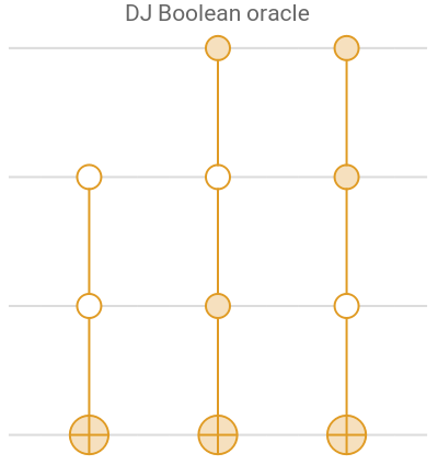
The quantum Deutsch–Jozsa algorithm can use two oracle types. The Boolean oracle acts on an n-qubit input register plus one ancilla qubit: it leaves the input unchanged and flips the ancilla exactly when the function evaluates to 1.
The above bit oracle acts as |x〉|y〉=|x〉|y⊕f(x)〉 where represents n-qubit case and the ancillary one (the last qubit)
U
f
|x〉
|y〉
Out[]=
|x〉|y〉 | DJ|x〉|y〉 | |x〉|y⊕f(x)〉 |
|1111〉 | |1111〉 | {1,1,1,1} |
|1110〉 | |1110〉 | {1,1,1,0} |
|1101〉 | |1100〉 | {1,1,0,0} |
|1100〉 | |1101〉 | {1,1,0,1} |
|1011〉 | |1010〉 | {1,0,1,0} |
|1010〉 | |1011〉 | {1,0,1,1} |
|1001〉 | |1000〉 | {1,0,0,0} |
|1000〉 | |1001〉 | {1,0,0,1} |
|x〉|y〉 | DJ|x〉|y〉 | |x〉|y⊕f(x)〉 |
|0111〉 | |0111〉 | {0,1,1,1} |
|0110〉 | |0110〉 | {0,1,1,0} |
|0101〉 | |0101〉 | {0,1,0,1} |
|0100〉 | |0100〉 | {0,1,0,0} |
|0011〉 | |0011〉 | {0,0,1,1} |
|0010〉 | |0010〉 | {0,0,1,0} |
|0001〉 | |0000〉 | {0,0,0,0} |
|0000〉 | |0001〉 | {0,0,0,1} |
We have highlighted all instances where the Boolean expression is true:
|x〉
boo
In[]:=
Boole[SatisfiabilityInstances[boo,{x,y,z},All]]
Out[]=
{{1,1,0},{1,0,1},{1,0,0},{0,0,0}}
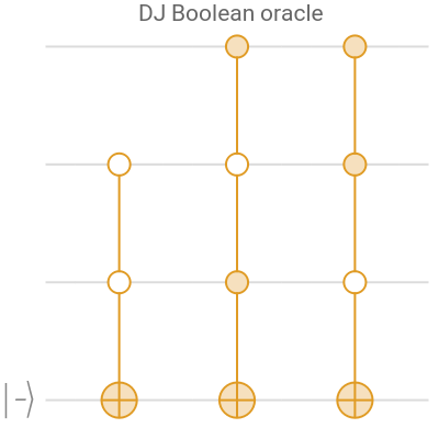
An important feature: if the ancilla is initialized in the minus state, the Boolean oracle leaves it unchanged and instead tags solutions by a negative phase on the corresponding n-qubit terms.
Out[]=
|x〉|y〉 | DJ|x〉|y〉 |
|111 − | |111 − |
|110 − | -|110 − |
|101 − | -|101 − |
|100 − | -|100 − |
|011 − | |011 − |
|010 − | |010 − |
|001 − | |001 − |
|000 − | -|000 − |
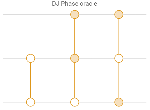
The Deutsch–Jozsa phase oracle uses no ancilla and applies a negative phase to input states that satisfy the function.
Out[]=
|x〉|y〉 | DJ|x〉|y〉 |
|111〉 | |111〉 |
|110〉 | -|110〉 |
|101〉 | -|101〉 |
|100〉 | -|100〉 |
|011〉 | |011〉 |
|010〉 | |010〉 |
|001〉 | |001〉 |
|000〉 | -|000〉 |
Deutsch-Jozsa Algorithm
Deutsch-Jozsa Algorithm
Putting it all together, the Deutsch-Jozsa circuit with the Boolean oracle is: prepare the input register in equal superposition and the ancilla in the minus state, apply the Boolean oracle, then measure the input register in the Pauli-X basis. If the outcome of measurements is only , declare constant; otherwise, declare balanced.
|〉
⊗n
+
Show the Deutsch–Jozsa circuit for the previously discussed Boolean function:
In[]:=
QuantumCircuitOperator["DeutschJozsa"[boo]]["Diagram"]
Out[]=
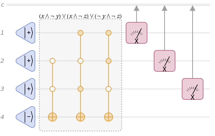
Pay close attention to the measurements. In Deutsch–Jozsa, the measurements are in the Pauli-X basis. The same circuit can also be presented in an equivalent form as follows.
In[]:=
({"H"->Range[4],"Z"->4}/*QuantumCircuitOperator["DeutschJozsaBooleanOracle"[boo]]/*{"H"->Range[3],{1,2,3}})["Diagram"]
For the Deutsch–Jozsa phase oracle, as noted, there is no ancillary qubit. The overall circuit is:
Find all constant and balanced Boolean functions on three input bits. (Constant: all 0s or all 1s; Balanced: four 1s and four 0s across the eight inputs.)
For three input bits (eight inputs): 70 balanced functions and 2 constant functions.
Bernstein-Vazirani Algorithm
We will discuss Bernstein-Vazirani algorithm. Bernstein–Vazirani finds a hidden n-bit string using one oracle call instead of n. Prepare the n input qubits in equal superposition and the extra “answer” qubit in a state that turns flips into phases. Query the bit oracle once; its action doesn’t store information in the answer qubit but kicks back a phase pattern onto the inputs that encodes the hidden string. Apply Hadamards to convert that phase pattern into a single basis state corresponding to the hidden string. Measure the inputs and read the string with certainty. The speedup comes from superposition, phase kickback, and interference, reducing queries from n to one.
Key Concepts
Key Concepts
◼
Oracle function
◼
Bernstein-Vazirani (BV) Algorithm
Statement of the Bernstein-Vazirani Problem
Statement of the Bernstein-Vazirani Problem
In many computer science problems, it is common to assume there is some kind of oracle function that is used in order to compute partial results for use in the rest of an algorithm. In practice, the oracle could be a database query or some similar operation.
Let’s consider a secret sequence of 0 and 1:
Check that the result is the same as the secret code:
Quantum Bernstein-Vazirani Algorithm
Quantum Bernstein-Vazirani Algorithm
Recall the secret sequence from before:
The quantum BV oracle for this sequence is given by:
In order to use this oracle to discover the secret code, only one query is necessary. Using the phenomenon of phase kickback, it is possible to send a uniform superposition of all possible sequences (as measured in the computational basis) and encode the solution in the three control qubits.
The full circuit would look like this:
Execute the above circuit and get the result:
It is clear that, in the new basis, the state is represented more compactly, and the idea of a uniform superposition with the answer qubit in the minus state is made explicit.
As before, in you look at the code above, we did a basis transformation.
The final step is measurements. Note we only measure n-qubits.
Therefore, the algorithm gives the secret code in only a single query.
The key feature of the BV algorithm is that the final measurement yields a single, definite result, the secret string. While this is elegant in theory, in practice, noise can interfere with the algorithm’s performance. In the next section, we will briefly discuss the impact of noise.
Effects of Noise
Effects of Noise
While solving the problem in only a single query to the quantum oracle is possible theoretically, real quantum circuits involve some errors caused by various effects. All of the previous circuits you have considered did not take this phenomena into account.
The following circuit defines the BV algorithm but introduces a noise channel just before the measurements can be performed. You might imagine this noise is from imperfect measurement or from the cumulative effect of previous errors in the circuit.
A noisy version of the previous circuit might look like this:
Notice that the measurement distribution now depends on the probability of the noise channels affecting each qubit:
If the so-called depolarizing noise channels affect the qubits with probability under 5%, the chance of returning the secret code is still quite high:
The following animation shows the effect of increasing the depolarizing probability:
As the noise rate increases, the probability of the intended outcome decreases. When noise reaches its maximum level, all outcomes occur with equal probability, meaning the noise effectively randomizes or smears the distribution of results.
Grover Search Algorithm
Key Concepts
Key Concepts
◼
Boolean function
◼
Grover Boolean oracle
◼
Grover Phase oracle
◼
Grover diffusion
Statement of the Grover Search Problem
Statement of the Grover Search Problem
Grover’s search is a core quantum algorithm. The task: given a Boolean function on n-bit inputs with one or more marked inputs (where the function returns True), find a marked input using as few oracle queries as possible.
Define a Boolean function
Now let’s examine its truth table:
Let’s count the number of possible combinations of variable values that yield True when supplied as arguments to the Boolean function
Grover’s key advantage can be illustrated as follows: by repeating the Grover circuit twice, the success probability can reach 100%, whereas a comparable classical strategy is about 20%.
Another subtlety of Grover’s algorithm is that there is an optimal number of Grover iterations to maximize the success probability. As the illustration shows, the classical success probability increases monotonically with more queries, while Grover’s success oscillates and can decrease if you go past the optimum.
Let’s dive in and examine the details of Grover’s algorithm. We will set up the register, define the oracle, apply the Grover iterate (oracle plus diffusion), and analyze how repeated iterations amplify the marked states to enable high-probability retrieval of the solution.
Grover oracle
Grover oracle
Grover’s algorithm commonly uses two oracle types: the Boolean oracle and the phase oracle. Both encode information about the solution to a Boolean function. In the Boolean oracle, the solution is written to an ancillary (target) qubit. In the phase oracle, there is no ancilla; the solution is encoded in the phase. Let’s examine them in more details.
Boolean oracle
Boolean oracle
Using the previous truth table, we can reproduce it with a quantum Boolean oracle. The oracle leaves the index register unchanged and flips the ancillary qubit exactly for inputs that satisfy the Boolean function, matching the table.
First, generate the corresponding Boolean oracle’s quantum circuit:
The diagram of the Boolean oracle:
Show how the oracle transforms states:
As one can see, the Boolean oracle circuit reproduce the same result as the classical ones.
Show the effect of the Boolean oracle on the new initial states:
One can see that the oracle introduces a relative phase only on the terms that are solutions of the Boolean function.
Let’s verify that the final states are physically identical to the initial ones, since the oracle introduced only a global phase (which has no observable effect).
As expected, only the solutions get a different phase shift. Note we have calculated that shift quantum mechanically.
Phase oracle
Phase oracle
Another common Grover oracle is the phase oracle. The key difference from the Boolean oracle is this: with a Boolean oracle, the solution is written to an ancillary (target) qubit; with a phase oracle, there is no ancilla and the solution is encoded as a phase. Let’s examine the phase oracle in more detail.
Create the corresponding phase oracle of the Boolean function:
The diagram of oracle:
As one can see, the oracle circuit reproduce the same result as the classical ones, but this time the solution information is in the phase.
Grover’s Algorithm
Grover’s Algorithm
The full Grover search operation looks like this:
The second block of gates is known as the Grover diffusion operator. The combination of the Boolean oracle and Grover diffusion operator are applied together in one iteration of the algorithm. To take advantage of the phase kickback introduced by the controlled gates, the circuit will need an initial set of gates and finally a measurement of the first three qubits.
One iteration of the Grover algorithm for the current example would look like this:
The measurement distribution for this circuit is shown below:
Recall that, for the states above, the Boolean function outputs are:
From the full measurement distribution, sum only the probabilities of inputs labeled True (1 in the above list).
As one can see, with the chance of around 65%, we can get the correct solution of the Boolean function by only one iteration of Grover.
Now what happens if two iterations are used instead of one?
The circuit is longer, but now the probability for obtaining the desired outcome is increased:
In this case, with the chance of most 100%, we can get the correct solution of the Boolean function by only two iterations of Grover.
We can also calculate the success probability given the number of Grover iteration:
As you can see, the probability rises then falls and rises again as more and more Grover iterations are applied.
Quantum Arithmetic
We will cover quantum arithmetic circuits centered on the Quantum Fourier Transform, showing how QFT enables addition and multiplication, how these operations are implemented in the Fourier basis, and how to transform to and from that basis.
Key Concepts
Key Concepts
◼
Discrete Fourier Transform
◼
Quantum Fourier Transform (QFT)
◼
Fourier (phase) Basis
◼
Phase adder
Discrete Fourier Transform and QFT
Discrete Fourier Transform and QFT
The discrete Fourier transform is a mathematical transformation that is very useful in processing data. It has many applications and is often employed when one wants to analyze signals over time.
The Quantum Fourier Transform maps an n-qubit computational-basis state to a uniform superposition whose phases encode the original index in Fourier order:
In fact, QFT is a basis change. For a general 2-qubit state with four amplitudes (ordered as 00, 01, 10, 11), the 2-qubit QFT applies a 4-point discrete Fourier transform to those amplitudes. Each basis component spreads over all four outputs with specific relative phases; the new four amplitudes are the Discrete Fourier Transform of the original four.
The circuit to implement a 3-qubit QFT is given below:
One can show that the overall effect of QFT (i.e. its matrix) is exactly the same as usual Fourier matrix:
Transforming a quantum state into the Fourier basis is exactly the action of the QFT on that state. Think of the QFT as the basis change to the Fourier basis.
Phase Basis Encoding
Phase Basis Encoding
As we discussed before, the computational basis is not the only way to encode classical information in a quantum state. Recall that the relative phase between two states can be experimentally distinguished. Thus, even if two states have the same probability to obtain outcomes in the computational basis, they are not the same state and will give different probabilities for outcomes in some other basis.
With this in mind, consider the following circuit:
The above circuit encodes an integer in n qubits. Here, the integer 1 is encoded in three qubits. In 3-bit binary, 1 is 001.
But how do you "read out" this phase information if all the measurements are performed in the computational basis? If you simply try to measure, the information encoded in the qubit phases is lost.
As you can see from the changing colors in the above plot, the information of the input state is transferred to information about the relative phases of each qubit (with respect to a uniform superposition in the computational basis). But that information is not accessible if measuring in the computational basis:
As you can see from the plot, the phase information is not immediately accessible in the computational basis. Instead, you must perform the inverse of the quantum fourier transform, and then measure.
By performing the inverse quantum Fourier transform, all of the phase information is now encoded in the computational basis. The measurement outcome is now the same as the number which was encoded in the phase basis:
With the phase basis and QFT in hand, you can implement quantum arithmetic circuits. The final state 001 matches the 3-qubit binary encoding of the integer 1.
Quantum Phase Adders
Quantum Phase Adders
This circuit first performs a quantum Fourier transform to get the input information into the phase basis, then applies an operation to add 3 in the phase basis, then performs an inverse quantum Fourier transform, and finally measures the results:
Find the measurement probabilities:
Given the outcome with maximum probability, determine the corresponding integer (using the bitstring-to-integer mapping):
Generic Addition
Generic Addition
Let’s walk through the above circuit step-by-step: Initialize the first three wires in 101 (which is 5) and the last three in 001 (which is 1). Apply QFT to the last three (to move them to the Fourier basis), use the phase adder to add in the Fourier basis, then apply the inverse QFT to return them to the computational basis. Recall the final result is encoded in the last three qubits.
With probability 1, the measured outcome of this circuit gives the state corresponding to 4 when the input states both correspond to 2.
Multiplication
Multiplication
The above circuit combines QFT and inverse QFT blocks with the multiplication subroutine in the Fourier basis.
Create the multiplication circuit:
Show the circuit diagram:
Show the expanded diagram up to the level 2:
As expected, you get 9 with 100% probability when running this circuit:
001100 bit-string corresponds to 12:
Quantum Phase Estimation Algorithm
We will discuss the Quantum Phase Estimation (QPE) algorithm. This algorithm estimates the eigenvlaues of a unitary by applying controlled powers of it to an eigenstate, imprinting the phase on ancilla qubits, then using the inverse quantum Fourier transform to read out a binary approximation; precision scales with the number of ancillas, enabling applications like factoring and eigenvalue estimation.
Key Concepts
Key Concepts
◼
Eigenvalue
◼
Eigenvector
◼
Quantum Fourier Transform
◼
Quantum Phase Estimation (QPE)
Eigenvectors and Eigenvalues
Eigenvectors and Eigenvalues
Eigenvectors and eigenvalues are concepts from the theory of linear algebra, and they are frequently used in analyzing the solutions of all sorts of mathematical models.
As an example, consider the matrix corresponding to the Pauli Z operator in the computational basis:
Check the matrix is Hermitian:
Check all eigenvalues are Real:
Of course, there is also a direct way of checking unitarity in the Wolfram Language:
Find the corresponding eigenphases:
Let’s consider a random unitary matrix:
Remember that any random generation follows a specific distribution. Here, the random unitaries are sampled uniformly from the unitary group (the Haar measure over n-dimensional unitary matrices).
Given above random unitary operator, let’s obtain its eigenvalues:
Quantum Phase Estimation: Simple Example
Quantum Phase Estimation: Simple Example
So far we computed eigenvalues classically. Quantum Phase Estimation uses phase kickback to extract an eigenstate’s phase, providing the information needed to recover the eigenvalues. For pedagogical purposes, consider the following unitary operator; we will use QPE to estimate its eigenphases.
Calculate the eigenvalues:
Calculate the eigenphases:
Let’s explore QFE for the unitary operator we generate above. Let’s consider the first eigenvector:
Prepare the target in the unitary’s first eigenstate. Initialize the control qubits in uniform superposition with Hadamards. Apply the sequence of controlled powers, then the inverse QFT, and measure the control register.
Execute the circuit and plot the measurement probabilities.
Compute the percentage error in the estimated phase (argument) of the first eigenvalue:
Quantum Phase Estimation: Complicated Example
Quantum Phase Estimation: Complicated Example
Visualize the overall Dirichlet kernel, and the individual kernels, for different linear combinations of eigenstates.
Consider the same circuit, but prepare the target qubit in a fixed (pedagogical) pure state chosen to mimic a random state, so we can illustrate the key effects clearly.
Plot the measurement probabilities for the control qubits.
We simulated the circuit without explicit measurement. After the unitary evolution, we traced out the target qubit to obtain the reduced state of the control register, then read off the computational-basis probabilities from that reduced state.
Now let’s obtain the overall Dirichlet kernel from simulations without assuming any knowledge of the unitary’s eigenstates or eigenphases. First, implement code that mimics experimental outcomes: a variable (randomResult) samples control-register measurement results according to the predicted probabilities each time the it is executed.
Calculate a smooth kernel distribution based on the data obtained above (after transforming it into the corresponding integers):
Note that the smooth distribution we obtained is the overall Dirichlet kernel.
As you can see, it has only one peak. Let’s increase our resolution by adding more control qubits, while preparing the target qubit in the same state:
Repeat the same steps to obtain the corresponding overall Dirichlet kernel.
Given new data, find the overall Dirichlet kernel
Now we can see two peaks clearly.
Let’s get two measurement results corresponding to the two peak we obtained:
Calculate the estimated eigenphases for the two peaks:
Compare the estimated values with the true values:
In practice, the situation can be more complex. If increasing the number of control qubits still yields no clear multiple peaks, the target’s initial state likely needs adjustment. With suitable state-preparation strategies, you can obtain informative outcomes. These techniques are beyond this course, but are worth exploring—the computational machinery is exactly what we’ve used above.
Shor’s Algorithm for Factorization
We will present a concise overview of Shor’s algorithm as a hybrid quantum–classical method for integer factorization. The classical stages reduce factoring to order finding and later convert the quantum output into nontrivial factors via greatest common divisors. The quantum core uses phase estimation on a modular multiplication unitary to extract periodicity, from which the order is inferred and factors are recovered with high probability. An illustrative example and operator construction clarify how the circuit is built and why it yields an efficient factoring procedure compared to known classical algorithms.
Key Concepts
Key Concepts
◼
Hybrid algorithm
◼
Shor’s algorithm
◼
Order finding problem
Factorization Through Order Finding
Factorization Through Order Finding
Efficient integer factoring matters in many applications (e.g., cryptography). For some special integers, fast classical methods exist. More generally, factoring can be reduced to an order-finding problem, for which there is an efficient quantum algorithm: Shor’s order-finding. In a hybrid approach, classical pre-processing reformulates factoring as order finding, the quantum routine solves that subproblem, and classical post-processing converts its output back to the factors. If both classical stages are efficient, this hybrid yields a faster overall factoring method than known classical algorithms.
Full algorithm
Full algorithm
The steps for Shor’s probabilistic algorithm to factor are as follows:
2
.2
.Otherwise, you have already found a nontrivial factor.
3
.1
.If is even, continue.
3
.2
.If is odd, the algorithm failed, and you must try with a new .
4
.2
.Otherwise, you must try with a new .
Example: Step-by-Step Factorization
Example: Step-by-Step Factorization
Verify that is neither even nor a prime number:
Check that and are coprime:
Compute the multiplicative order of modulo :
Note that above step is the one that has a quantum subroutine. We will discuss it later.
Order Finding with a Quantum Circuit
Order Finding with a Quantum Circuit
Remember that a quantum operator can be specified as a matrix that defines its action on states. What happens if you try to define a multiplication operator using the most straightforward approach? Is such an operator unitary?
You can mathematically specify such a matrix without difficultly; however, the resulting matrix is not unitary. This is mathematically fine, but you cannot implement such an operation using any rules consistent with quantum mechanics. Thus, the simplest approach to define a quantum operator for this problem is ruled out.
Instead, specify an operator such that it has the expected action on elements which are less than , and leaves elements through the maximum size of the Hilbert space unchanged.
Therefore, the desired unitary operator can be implemented as follows:
Notice that this operator raised to the multiplicative order of modulo gives the identity operator:
Consider the following phase estimation circuit for the unitary operator that implements multiplication by modulo (in this case 13 modulo 15):
Compute the measurement distribution:
Plot the distribution:
Post-Processing the Eigenvalue Estimations
Post-Processing the Eigenvalue Estimations
Exploring the Details
Exploring the Details
First, let’s label the new basis elements according to their eigenvalues (and an arbitrary index, since there are repeated eigenvalues):
Now, each new basis vector has an arbitrary index and you can see its corresponding eigenvalue:
This (perhaps surprising) fact is what allows the quantum phase estimation algorithm to sample uniformly from the distinct eigenvalues.
Quantum Key Distribution: BB84 scheme
BB84 (named after Bennett and Brassard's 1984 paper) is a quantum protocol for securely establishing a shared secret key between two parties. It is the earliest and most well-known example of Quantum Key Distribution (QKD), and it uses properties of quantum mechanics, such as the fact that measuring a quantum state disturbs it, to detect any eavesdropping and ensure the secrecy of the generated key.
Key Concepts
Key Concepts
◼
BB84 protocol.
◼
Quantum Key Distribution
One-time pad encryption
One-time pad encryption
In this section, we briefly review the one-time pad encryption by using a secret key, securely shared between two parties (e.g., Alice and Bob). We let Alice and Bob share the same secret key securely. Once they have that key, they use it in an ordinary classical one-time pad encryption.
First, Alice and Bob need a way to turn text into bits. Let’s define a function that is doing just that.
Define a function that returns the ASCII bits of a string:
When you give it a string like “Wolfram”, it takes each character, finds its ASCII code (a number that represents that character), and then converts that number into its binary representation, that is, a sequence of zeros and ones.
Select a secret key (shared securely between Alice and bob):
The output is a list of lists: one list of seven bits for each character. This list of bit blocks is what both Alice and Bob possess as their shared secret key.
Then Alice prepares the message she wants to send, which here is the word “Quantum”.
Select a message (Alice wants to send it to Bob):
Now Alice has two aligned lists: one is the message bits, one is the key bits, both the same length, with each character of the message lined up with a corresponding character of the key. To encrypt, Alice combines the message bits with the key bits using the bitwise XOR operation. XOR is a very simple rule on individual bits: if the two bits are the same, the result is zero; if they are different, the result is one. The result is a ciphertext that looks like nonsense if you try to interpret it as plain text, and without the key, it gives no information about the original message.
Generate a ciphertext by taking the XOR of each bit of the message with each bit of the secret key (Alice does this, and send the ciphertext to Bob):
Alice then sends this ciphertext over the classical channel to Bob. An eavesdropper can see the ciphertext, but without the key, the one-time pad guarantees that the message is information-theoretically secure, provided the key is truly random, at least as long as the message, and used only once. When Bob receives the ciphertext, he decrypts it using the exact same operation: bitwise XOR with the same key.
Decode the ciphertext by taking the XOR of each bit of it with each bit of the secret key (Given Alice message, Bob does this step):
Show the text of the decoded text:
So, in plain language, Alice and Bob shared a secret string of bits. Alice turned her message into bits, combined it with the secret bits using XOR to produce an encrypted bit string, and send that to Bob. Bob used the same secret bits and the same XOR operation to reverse the process and get the original message back.
Bennett-Brassard quantum solution (BB84)
Bennett-Brassard quantum solution (BB84)
As an example of a quantum key distribution (QKD), we consider BB84 protocol. It starts with Alice. She decides she’s going to send nine qubits to Bob. Note that the number of qubits (here nine) is completely your choice and not special to BB84 at all. For each qubit, Alice needs two random choices: which bit she wants to encode (zero or one), and which basis she wants to use to encode it. In BB84, there are two possible bases: the Z basis and the X basis. We will first choose nine random bits for Alice, and then nine random bases, each either Z or X. So, for each position from one to nine, Alice now has a pair: a bit and a basis.
Generate bases and bits of Alice randomly for nine qubits:
Depending on what bit and what base, Alice follows the following protocol for sending a qubit to Bob:
Visualize Alice’s protocol:
Also recall the common convention for the computational basis:
Next, take every pair of Alice’s random bit and basis and pass them through Alice’s sending rules. That produces a list of nine actual qubit states: some of them are plain zero or one in the Z basis, and some are the plus or minus states in the X basis.
Therefore, given Alice’s bit and bases that are generated randomly, she will send Bob these qubits:
The above sequence of qubits is what Alice will physically send down the quantum channel to Bob.
Now it’s Bob’s turn. Bob doesn’t know which basis Alice used for each qubit, so he follows the BB84 rule: for every qubit he receives, he randomly chooses a basis of his own, again either Z or X.
Bob randomly generate a sequence of either Z-basis or X-basis of measurement:
It means, Bob applies the measurement operators in above bases on qubits he relieved from Alice. Each measurement destroys the original qubit state and produces an outcome in the basis Bob chose. To see a specific “run” of what could happen, we will simulate one possible set of outcomes, giving a concrete basis state for each qubit, such as the plus or minus state in X, or the plus or minus state in Z.
Generate measurement objects for Bob:
Return one possible realization of Bob' s series of measurements (note some will always return the same result, some randomly, depending on what Alice' s qubit is and what direction Bob measures):
Once Bob has a list of measurement outcomes, he needs to convert these into bits. The convention in this code is simple: whenever he gets the “plus” outcome in either basis, he calls that bit zero; whenever he gets the “minus” outcome in either basis, he calls that bit one.
At this stage, Alice has her original sequence of bits and bases; Bob has his bits and his bases. Many of Bob’s bits will not match Alice’s bits, because sometimes he measured in the “wrong” basis. That is the core of BB84: if Bob chooses a different basis from Alice, his result is completely random and carries no reliable information about Alice’s bit.
The next step is the classical sifting process. Alice and Bob now talk over a normal (but authenticated) classical channel. Importantly, they do not reveal their bits. Instead, they reveal only the bases they used for each position. For each index from one to nine, they compare Alice’s basis and Bob’s basis. If they used the same basis, they keep that position; if they used different bases, they discard it.
Zip together Alice’s bits, Alice’s bases, and Bob’s bases into triples, then select only the triples where Alice’s basis equals Bob’s basis:
Alice extracts her bits from these surviving triples to get her secret key. Bob does the same with his bits: he takes his bits from the positions where the bases match.
Both resulting lists of bits are identical! Alice and Bob have successfully distilled a shorter, but shared, secret key out of the original nine transmissions.
The key that came out is shorter than the number of qubits Alice sent. That’s expected. Whenever Bob happened to guess the wrong basis, that position got thrown away. In the long run, about half the positions survive. If Alice and Bob want a key of a certain length, they just keep running this process, Alice sending more qubits, Bob measuring with random bases, and both of them doing the public basis comparison and discarding mismatches, until the number of agreed positions reaches the desired length. This can be implemented as follows.
This can be implemented as follows. Take the current partial keys for Alice and Bob, runs one more “round” of the protocol for a single qubit (choosing a random bit and basis for Alice, generating a qubit, choosing a random basis for Bob, measuring, mapping Bob’s outcome to a bit), then checks if the bases matched. If they did, append the new bit to both Alice’s and Bob’s keys; if not, leave the keys unchanged. Then, using NestWhile, repeatedly call this function, starting from empty keys, until Alice’s key reaches a length of five bits.
For example, the key length is set as 5 bits in the following:
All of this is the “quantum” front end that you can connect to the one-time pad we discussed about earlier. BB84 gives Alice and Bob a shared random key, built in such a way that any eavesdropping would disturb the statistics of their measurements and be detectable. Once they have that key, they can use it exactly as in the one-time pad example: combine it with a message using XOR to encrypt, and combine again with the same key to decrypt.
Acknowledgment
A portion of this book builds on an early draft prepared by John McNally of Wolfram Research during his work on this project. Many of the ideas and their presentation grew through countless conversations with colleagues at Wolfram Research, including Nikolay Murzin, Bruno Tenorio, and Sebastian Rodriguez. I would also like to express my gratitude to Stephen Wolfram, founder and CEO of Wolfram Research, for his steady support throughout the years I’ve led the quantum initiative. Finally, my heartfelt thanks go to the late Michael Trott (friend, mentor, and teacher) who, sadly, passed away before I completed this draft. He is deeply missed.
CITE THIS NOTEBOOK
CITE THIS NOTEBOOK
Introduction to quantum computing: part 2
by Mads Bahrami
Wolfram Community, STAFF PICKS, December 9, 2025
https://community.wolfram.com/groups/-/m/t/3587994
by Mads Bahrami
Wolfram Community, STAFF PICKS, December 9, 2025
https://community.wolfram.com/groups/-/m/t/3587994