ABSTRACT (original article): Let be the set of sum-product pairs, where is the sumset and is the product set We construct a dataset consisting of 1162868 sets whose sum-product pairs are at least 84% of for each . Notably, we do **not** see evidence in favor of Erdős’s Sum-Product Conjecture in our dataset. For , we prove the exact value of . We include a number of conjectures, open problems, and observations motivated by this dataset, a large number of color visualizations. CITATION (original article): Kevin O’Bryant (2024), Visualizing the Sum-Product Conjecture, arXiv:2411.08139. https://doi.org/10.48550/arXiv.2411.08139
SPP(n)
{(|A+A|,|AA|):A⊆,|A|=n}
A+A
{a+b:a,b∈A}
AA
{ab:a,b∈A}.
SPP(n)
n≤32
n≤6
SPP(n)
The sumset of a set of integers is the set , and the product set is . By elementary combintorics, both and are between and . One of the most worked-upon conjectures in additive number theory is Erdös’s Sum-Product Conjecture: For all , if is large enough, then at least one of is at least .
A+A
n
{a+b:a∈A}
AA
{ab:a,b∈A}
|A+A|
|AA|
2n-1
n(n+1)/2
ϵ>0
n
|A+A|,|AA|
2-ϵ
n
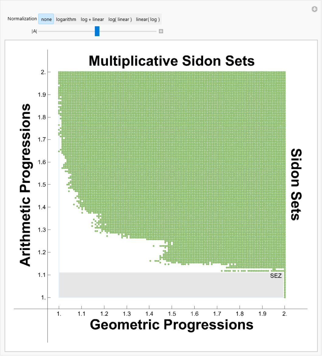
In “Visualizing the Sum-Product Conjecture” I computed as many sum-product pairs for each up to 32 as I could manage, with constrained to the positive integers. This dataset is certainly incomplete but contains at least 7/8-ths of the conceivable sum-product pairs for each .
(|A+A|,|AA|)
n=|A|
A
n
One can certainly stare at the unnormalized pairs, but the sum-product conjecture just concerns pairs that are extremely close to (1,1), the lower-left corner of our picture.
A more interesting picture is to normalize with a base- logarithm, i.e., the pairs . Now, the Sum-Product Conjecture says that as , the sum-product pairs must congregate along the northern or eastern edge of our picture. However, the pictures show that not only are the points not drifting north and east, but the lower envelope is actually moving south and west! This suggests that the Sum-Product Conjecture may be false (or that is too small).
The combinatorial upper and lower bounds are approximately/2 and , and the effect of these factors of 2 shows up in these images as stretching the points away from the center as increases. So perhaps this explains the drift south and west for small .
n
(|A+A|,|AA|)
log
n
log
n
n->∞
n=32
The combinatorial upper and lower bounds are approximately
2
n
2n
n
n
It is known that if the product set is too small, then the sumset must be extremely large, this region is labelled as SEZ on our pictures. Solymosi has proved that a particular triangle cannot contain any limit points in its interior, and this triangle is marked in our pictures as the “Solymosi Void”.
To compensate for those factors of 2 in the upper and lower bounds, we can normalize better. We can find find linear functions ,, so that
ϕ
1
ϕ
2
ϕ
3
log
n
ϕ
1
log
n
n(n+1)
2
ϕ
1
n(n+1)
2
log
n
ϕ
2
log
n
ϕ
2
n(n+1)
2
ϕ
3
log
n
ϕ
3
log
n
n(n+1)
2
We show all of these normalizations in our images, and they all show sum-product pairs getting further south and further west, with more drift as increases.
n
Conjecture: For every set of positive integers, .
A
A+A*AA>=A
1
2
3
|
This conjecture is supported by our data, does not imply Erdös’s Sum-Product Conjecture, and seems to old for every set , not merely as .
A
|A|->∞
In[]:=
Get[FileNameJoin[{NotebookDirectory[],"SP.mdata"}]];SP[5]
Out[]=
{{9,14},{15,9},{12,12},{15,12},{13,12},{11,15},{14,12},{10,14},{15,11},{12,14},{15,14},{13,14},{14,14},{11,12},{10,15},{12,13},{12,15},{15,13},{15,15},{13,13},{13,15},{11,14},{14,13},{14,15},{15,10},{10,12},{9,15}}
Normalizing Functions
In[]:=
none[k_,x_]:=;K1[k_,x_]:=N+(2k-1)Logk,k(1+k)-Log[k,2k-1]+Logk,x+Log[k,x];L[n_,x_]:=N[Log[n,x]];K2[n_,x_]:=NLogn,x-;K3[n_,x_]:=NLog[n,x]+1+;normy[0]=none;normy[1]=L;normy[2]=K1;normy[3]=K2;normy[4]=K3;fromstring["none"]=0;fromstring["logarithm"]=1;fromstring["log + linear"]=2;fromstring["log( linear )"]=3;fromstring["linear( log )"]=4;
2x+4-7k+
2
k
2-3k+
2
k
4-7k+
2
k
2-3k+
2
k
-1
Binomial[k-1,2]
1
2
k(1+k)
2
-1
Binomial[k-1,2]
4k-2
1+k
2n
n-2
3
2
n
n-2
Log[n]
Log[n(1+n)]-Log[-2+4n]
Log[-1+2n]
Log[-2+4n]-Log[n+]
2
n
In[]:=
SolymosiVoid={Graphics[{LightPink,Opacity[0.5],Polygon[{{1,1},{1,2},{3/2,1},{1,1}}]}],Graphics[{Dashed,Red,Line[{{1,1},{1,2},{3/2,1},{1,1}}]}],Graphics[Rotate[Text[Style["Solymosi Void",Medium],{1.35,1.2}],ArcTan[-2]]]};
In[]:=
SEZ[k_]:=Module[{corner=If[k==3,{1.6,1.6},N[{K1[k,k(k+1)/2-Max[3/4,(1-1/k)]],K1[k,3k-3-Max[3/4,(1-1/k)]]}]]},{Graphics[{Black,Text["SEZ ",corner,{1,1}],RGBColor[0,0.05,0],Opacity[0.1],Rectangle[{1,1},corner]}]}];SEZ[normalizer_,k_]:=Module[{corner=If[k==3,{1.6,1.6},N[{normalizer[k,k(k+1)/2-Max[3/4,(1-1/k)]],normalizer[k,3k-3-Max[3/4,(1-1/k)]]}]],start=normalizer[k,2k-1]*{1,1}},{Graphics[{Black,Text["SEZ ",corner,{1,1}],RGBColor[0,0.05,0],Opacity[0.1],Rectangle[start,corner]}]}];background=ListPlot[{},AspectRatio->1,PlotStyle->Medium,PlotRange->{{0.95,2.05},{0.95,2.05}},Ticks->{Range[1,2,0.1],Range[1,2,0.1]}];box=Graphics[{LightBlue,Line[{{1,1},{1,2},{2,2},{2,1},{1,1}}]}];sidelabels=Graphics[{Text[Style["Geometric Progressions",Bold,Large],{1.5,0.88}],Text[Style["Multiplicative Sidon Sets",Bold,Large],{1.5,2.05}],Rotate[Text[Style["Arithmetic Progressions",Bold,Large],{0.85,1.5}],Pi/2,{0.85,1.5}],Rotate[Text[Style["Sidon Sets",Bold,Large],{2.05,1.5}],-Pi/2,{2.05,1.5}]}];
In[]:=
Clear[image];image[k_,n_Integer]:=image[k,n]=Module{pts,pic,sides},pts=Map[normy[k][n,#]&,SP[n]];pic=ListPlotpts,AspectRatio->1,PlotStyle->ColorData["Rainbow"],PointSize,PlotRange->{{0.80,2.10},{0.80,2.10}};Show[background,If[k!=0,SolymosiVoid,Graphics[]],SEZ[normy[k],n],box,pic,sidelabels,PlotRange->{{0.80,2.10},{0.80,2.10}},ImageSize->500];
n-3
29
0.06
Log[1+Length[pts]]
In[]:=
image[k_,33]:=image[k,33]=Module{pts,pic,onepic,maxn=32},Do[pts[n]=Map[normy[k][n,#]&,SP[n]],{n,3,maxn}];Doonepic[n]=ListPlotpts[n],AspectRatio->1,PlotStyle->ColorData["Rainbow"],PointSize[Small],{n,3,maxn};pic=Table[onepic[n],{n,maxn,3,-1}];Show[background,If[k>0,SolymosiVoid,Graphics[]],box,pic,sidelabels,PlotRange->{{0.80,2.10},{0.80,2.10}},Ticks->{{{1,"1.0"},{1.1`,"1.1"},{1.2`,"1.2"},{1.3`,"1.3"},{1.4`,"1.4"},{1.5`,"1.5"},{1.6`,"1.6"},{1.7`,"1.7"},{1.8`,"1.8"},{1.9,"1.9"},{2.`,"2.0"}},{{1,"1.0"},{1.1`,"1.1"},{1.2`,"1.2"},{1.3`,"1.3"},{1.4`,"1.4"},{1.5`,"1.5"},{1.6`,"1.6"},{1.7`,"1.7"},{1.8`,"1.8"},{1.9,"1.9"},{2.`,"2.0"}}},ImageSize->500]
n-3
29
In[]:=
Monitor[Do[image[k,n],{k,0,4},{n,3,33}],{k,n}]
Manipulate[image[fromstring[k],n],{{k,"none","Normalization"},{"none","logarithm","log + linear","log( linear )","linear( log )"}},{{n,16,"|A|"},3,33,1},SaveDefinitions->True]
Out[]=
CITE THIS NOTEBOOK
CITE THIS NOTEBOOK
Visualizing the sum-product conjecture
by Kevin O’Bryant
Wolfram Community, STAFF PICKS, July 5, 2025
https://community.wolfram.com/groups/-/m/t/3492137
by Kevin O’Bryant
Wolfram Community, STAFF PICKS, July 5, 2025
https://community.wolfram.com/groups/-/m/t/3492137