The purpose of this project is to investigate the gravitational lensing effect in the Wolfram Model. To do this we generate a causal graph by random sprinkling and then perturb the graph by adding local fluctuations in the edge density of the graph. We then investigate how this perturbation changes the shape of the light cone, as well as the light flux. We find that it is possible reproduce gravitational lensing in the Wolfram Model.
Introduction
Introduction
In a classical spacetime, light will follow a null geodesic. That is, the path where all infinitesimal points are null separated. This corresponds to the edge of the causal cone. In the Wolfram Model, we can find the interior of the light cone in much the same way by finding the set of vertices that are causally connected to a given source vertex. The light cone is then the boundary of that subgraph.
Causal Foliation
Causal Foliation
A causal foliation is a way to partition a causal graph into sets of point, which corresponds to timelike hypersurfaces. We can define the first layer of the foliation as all the vertices with no incoming edges. From here, we define a causal layer as the set of vertices with the same shortest distance to a vertex in the first causal layer [1].
Plot of a 1+1 spacetime with the fourth causal layer highlighted
In[]:=
g=generateFlatSpacetime[500,2,0.2];HighlightGraph[g,getHyperSurface[g,4]]
Out[]=
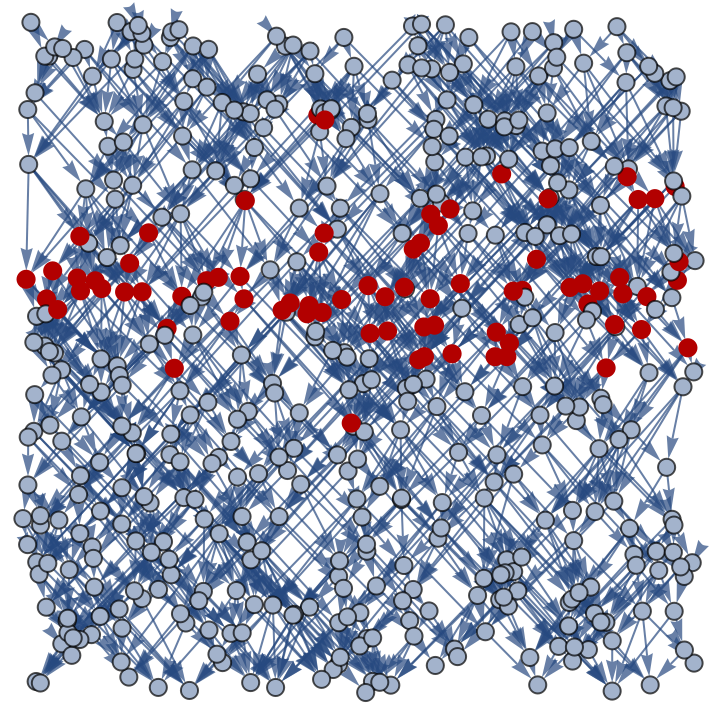
We do the same, but add a perturbation in the middle of the graph.
In[]:=
modifiedGraph=getPerturbedGraph[g,0.23,10];HighlightGraph[modifiedGraph,getHyperSurface[modifiedGraph,4]]
Out[]=
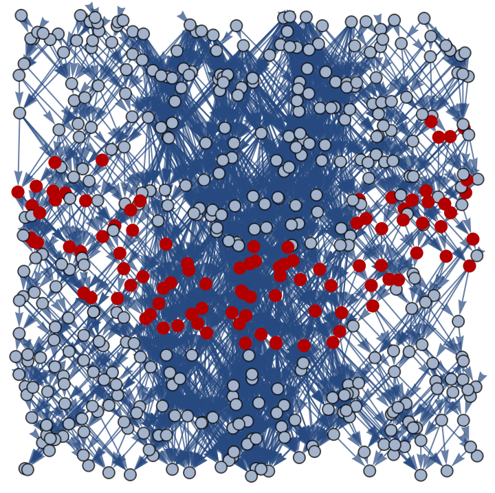
Comparing the two causal layers, we see how adding local edge density, will change the causal foliation and effectively cause the spacetime to curve, in a similar way that a mass fluctuation will cause the spacetime to curve in general relativity.
Dimension and Curvature Estimation
Dimension and Curvature Estimation
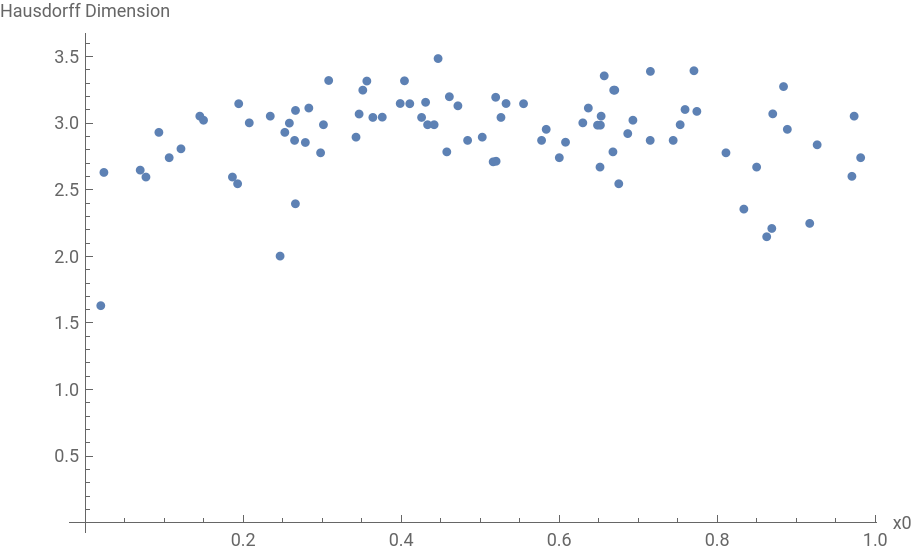
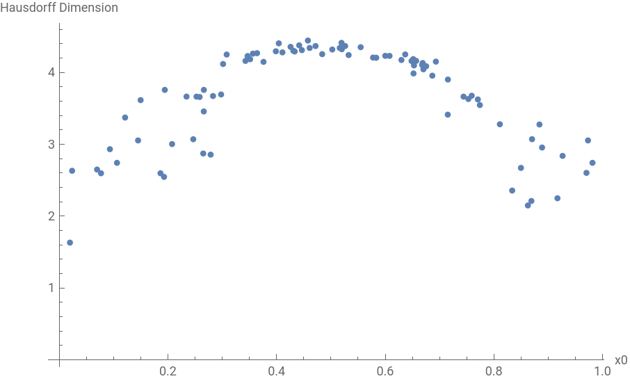
We use the resource functions WolframHausdorffDimension and WolframRicciCurvatureScalar to estimate the dimension of the causal graph. For the causal graphs above, we find the dimension as a function of the spatial coordinate for the unperturbed and perturbed graphs respectively:
And for the curvature
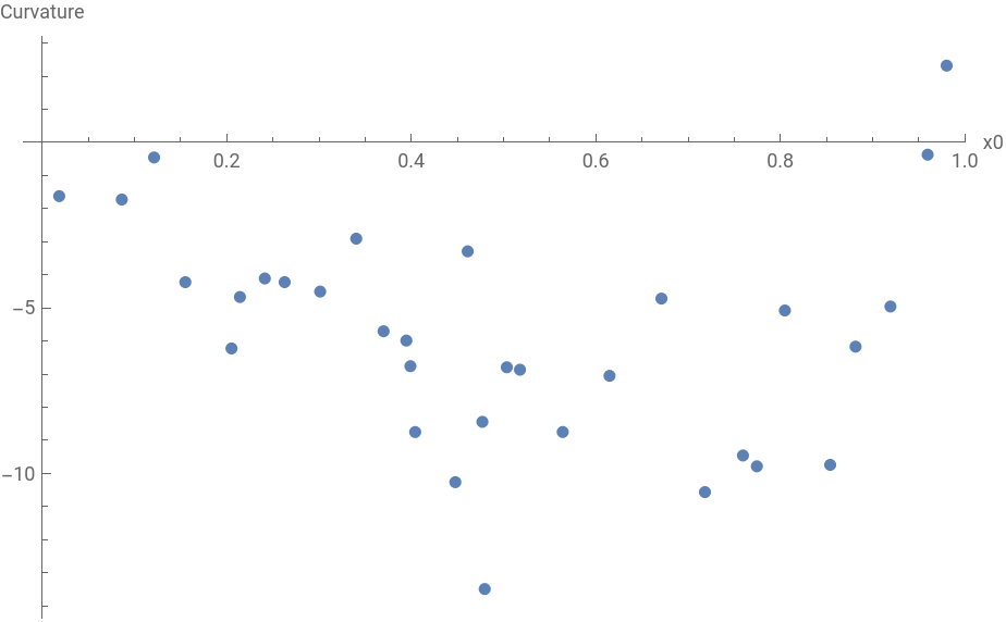
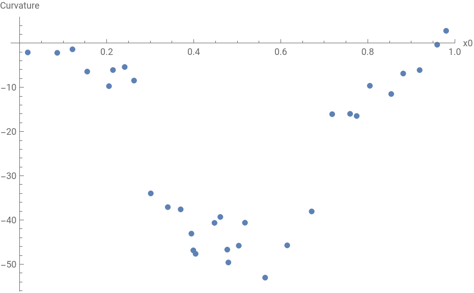
So we see how the perturbation affects both the dimension and the curvature. When calculating the dimension, we assume that the curvature is 0. When calculating the curvature, on the other hand, we assume the dimension to be a fixed integer value.
The Horismos
The Horismos
We define the Horismos, or the light cone, as the set of points traced out by by following all possible null geodesics starting at some initial source vertex. In practice we calculate the Horismos at some specific time by taking the intersection of the vertices that are causally connected to the initial vertex with the vertices in a specific causal layer. Next, we take the spatial projection of these vertices and use the ConvexHullMesh function to find the convex boundary of these points. With this we get a result of the following form in 2+1 dimensions. This is the only time in the calculations, where we use the coordinate information of the vertices.
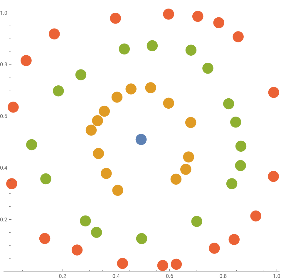
This plot shows the spatial projection of the vertices in the Horismos. Points with the same color correspond to vertices that belong in the same causal layer.
Preliminary Tests
Preliminary Tests
Before running the actual computation, we need to test a few things first. For all of the following calculations, the uncertainties are found by finding the variance over a statistical ensemble of different sprinklings.
Convergence to Circular Horismos
Convergence to Circular Horismos
In order to estimate the resolution needed to achieve results similar to those in the continuum case, we have to look at when the horismos in a flat spacetime has an approximate circular form. We vary the total number of points in the sprinkling, N, and calculate the mean absolute deviation of the radii of the vertices in a layer of the horismos. This means that a small value of the mean absolute deviation corresponds to a set of points that approximately defines a circle. The result is the following
This shows the mean absolute deviation of the radii of the vertices in the horismos of a layer in the causal graph as a function of the total number of vertices. The uncertainties are found by finding the variation of many different sprinklings. This shows that for N=3000, we find light cones that are good enough circular approximations that we can investigate how fluctuations perturb the circular shape.
Using this result, we will be working with causal graphs that have around 3000 vertices, as a higher number of vertices means that the calculations will become very slow.
Dimension Fluctuation vs Perturbation Strength
Dimension Fluctuation vs Perturbation Strength
In order to test whether the perturbation method, introduced in this project is well behaved, it is useful to see that changing the strength parameter in the function will not change the system too violently. The perturbation strength determines how many the edge density added in the perturbed region of the graph.
We plot the difference in dimension as a function of the perturbation strength. There is a large increase in dimension for small values, since we add more edges and therefore connect more vertices with shorter paths. The small decrease for large values of the perturbation strength is likely due to edge effects, since the edge effectively is closer in the foliation when we increase the connectivity.
We can conclude from this test that the most dramatic effect is for values of the perturbation strength <0.5, so this is where we should concentrate the measurements.
Dimension Fluctuation vs Number of Vertices
Dimension Fluctuation vs Number of Vertices
We plot the dimension fluctuation of a perturbation of a given strength against the number of of vertices in the causal graph, to see whether more points has an effect on the dimension difference.
From this plot we can see that the variation for different sprinklings is much higher than any overall effect on the dimension difference for higher number of vertices. For this reason, we can effectively treat the fluctuation strength as constant in the number of vertices.
Results
Results
Shape of the Horismos
Shape of the Horismos
In this experiment we look at the change in the shape of the causal slice of the horismos as we vary the strength of the perturbation. The idea is that as the perturbation becomes stronger, we get a more curved causal layer, which leads to a distorted light cone.
Here we see a light cone for a flat spacetime (blue) along with the light cone from the same source vertex in the perturbed spacetime (orange). This shows how the light is effectively “bent” when near the perturbed region of the spacetime.
We want to find a quantitative way to measure how much the horismos slice is distorted. To do this we calculate the difference in the mean absolute deviation of the radii of the points in the slice of the horismos. We find the following for the difference in the mean absolute deviation for the original and for the perturbed graph as a function of the curvature and the dimension difference.
We can also simply plot the dimension difference against the curvature difference.
The Curvature difference and the dimension difference. We see that the dimension difference remains mostly constant while the curvature changes more dramatically.
Plotting the dimension difference against the curvature difference, we see that after a certain threshold, the dimension remains more or less constant as we vary the curvature. This means that it might in principle be possible to change the curvature without affecting the dimension dramatically.
Spatial Distribution of Light Flux
Spatial Distribution of Light Flux
For this experiment we imagine a light source in one end of the causal graph (yellow vertices). This source is extended in one spatial direction and is continuously sending out a light signal. For a given causal layer, corresponding to a particular time, we count how many of the vertices in the horismoi have reached the other end of the causal graph (the red vertices). This is similar to the light flux that an observer at this part of the causal graph would measure.
A flat 2+1 spacetime sprinkling. The yellow vertices will correspond to the events where light is emitted. The red vertices correspond to the place where the light is observed.
For a particular causal layer (corresponding to a particular spacelike hypersurface) we measure the spatial distribution of the light flux at the observed (red) vertices, coming from the source (yellow) vertices. In the flat spacetime case, we would expect a homogenous distribution (perhaps with some edge effects). If we however, perturb the spacetime by adding more edges in one side of the graph, we should expect the distribution to be higher in one end than the other, corresponding to the bending of light.
Here we see the approximately flat spatial distribution of the light observed at the observer (red) points on the original graph along with the distribution on the perturbed graph. The increase in the flux around the edges, since some vertices will be counted as edges because the real edges are outside of the graph. The orange distribution corresponds to the change due to the perturbation on the left hand side. We see clearly how this leads to an increase of the flux on the left hand side, which would correspond to a bending of light around the curvature fluctuation.
Calculations
Calculations
The following is the code to produce the results showed earlier. Note however, that most of these computations take a long time to run.
Tests:
Tests:
Results
Results
Concluding remarks
Concluding remarks
In this project, I have managed to reproduce something similar to the gravitational lensing effect in the Wolfram Model. I was not able to detect a difference between a curvature and a dimensional fluctuation as we have found that we can always model a small curvature fluctuation with a large dimension fluctuation. This analysis has been done in a way that is almost coordinate independent. It would be interesting to completely remove the need for the vertices to have coordinate information, as this would allow us to perform the same analysis from this project, on a causal graph generated by an updating rule.
Keywords
Keywords
◼
Gravitational Lensing
◼
Spacetime
◼
Dimension
◼
Horismos
◼
Sprinkling
Acknowledgment
Acknowledgment
I would like to thank Jonathan Gorard and Yorick Zeschke for their excellent explanations and advice. I would also like to thank all the other students in the physics track for making the summer school such a fun and enjoyable experience.
References
References
◼
[1]: Jonathan Gorard (2020): “Some relativistic and gravitational properties of the Wolfram Model”. ArXiv preprint available at: https://arxiv.org/abs/2004.14810
◼
[2]: Jonathan Gorard (2020): “Algorithmic causal sets and the Wolfram model”. ArXiv preprint available at: https://arxiv.org/abs/2011.12174
◼
[3] Stephen Wolfram (2020): A Class of Models with the Potential to Represent Fundamental Physics. Complex Syst. 29(2), doi:10.25088/complexsystems.29.2.107. Available at https: //www.complex-systems.com/abstracts/v29_i02_a01/