Introduction:In this work we will look at a definite integral of the arctangent function expressed in terms of the log-gamma function.(tanh(xtan(t)))cot(t)t=πlogwhere Re(x)>0.
π/2
∫
0
-1
tan
1
2
ΓΓ+
1
4
x
π
3
4
ΓΓ
3
4
4x+π
4π
Here we define the integrand and the log gamma closed form solution
Here we define the integrand and the log gamma closed form solution
In[]:=
arctanl[x_]:=ArcTan[Tanh[xTan[t]]]Cot[t]
In[]:=
arctanr[x_]:=πLog
1
2
GammaGamma+
1
4
3
4
x
π
GammaGamma
3
4
π+4x
4π
Here we look at the numerical integral of the arctangent function for x = 1, π, π/2, π/4 and π/8
Here we look at the numerical integral of the arctangent function for x = 1, π, π/2, π/4 and π/8
In[]:=
arctanln[x_]:=NIntegrate[ArcTan[Tanh[xTan[t]]]Cot[t],{t,0,π/2}]
In[]:=
arctanln[1]
Out[]=
0.94262
In[]:=
arctanln[π]
Out[]=
1.7257
In[]:=
arctanln[π/2]
Out[]=
1.23023
In[]:=
arctanln[π/4]
Out[]=
0.804839
In[]:=
arctanln[π/8]
Out[]=
0.483061
Here we look at the equivalent numerical values for the log gamma function at x = 1, π, π/2, π/4 and π/8
Here we look at the equivalent numerical values for the log gamma function at x = 1, π, π/2, π/4 and π/8
In[]:=
arctanr[1]//N
Out[]=
0.94262
In[]:=
arctanr[π]//N
Out[]=
1.7257
In[]:=
arctanr[π/2]//N
Out[]=
1.23023
In[]:=
arctanr[π/4]//N
Out[]=
0.804839
In[]:=
arctanr[π/8]//N
Out[]=
0.483061
Here we will look at the closed form solutions of the integral for x = 1, π, π/2, π/4 and π/8
Here we will look at the closed form solutions of the integral for x = 1, π, π/2, π/4 and π/8
In[]:=
arctanr[1]//FullSimplify
Out[]=
1
2
GammaGamma+
1
4
3
4
1
π
GammaGamma+
3
4
1
4
1
π
In[]:=
arctanr[π]//FullSimplify
Out[]=
1
2
In[]:=
arctanr[π/2]//FullSimplify
Out[]=
1
2
GammaGamma
1
4
5
4
2
Gamma
3
4
In[]:=
arctanr[π/4]//FullSimplify
Out[]=
1
2
Gamma
1
4
π
Gamma3
4
In[]:=
arctanr[π/8]//FullSimplify
Out[]=
1
8
2
2
π
4
Gamma
1
4
8
Gamma
3
8
Here we will put the examples together for x = 1, π, π/2, π/4 and π/8
Here we will put the examples together for x = 1, π, π/2, π/4 and π/8
In[]:=
{Integrate[arctanl[1],{t,0,π/2}],arctanr[1]}
Out[]=
ArcTan[Tanh[Tan[t]]]Cot[t]t,πLog
π
2
∫
0
1
2
GammaGamma+
1
4
3
4
1
π
GammaGamma
3
4
4+π
4π
In[]:=
{Integrate[arctanl[π],{t,0,π/2}],arctanr[π]}//FullSimplify
Out[]=
ArcTan[Tanh[πTan[t]]]Cot[t]t,πLog[3]
π
2
∫
0
1
2
In[]:=
{Integrate[arctanl[π/2],{t,0,π/2}],arctanr[π/2]}//FullSimplify
Out[]=
ArcTanTanhπTan[t]Cot[t]t,πLog
π
2
∫
0
1
2
1
2
GammaGamma
1
4
5
4
2
Gamma
3
4
In[]:=
{Integrate[arctanl[π/4],{t,0,π/2}],arctanr[π/4]}//FullSimplify
Out[]=
ArcTanTanhπTan[t]Cot[t]t,πLog
π
2
∫
0
1
4
1
2
Gamma
1
4
π
Gamma3
4
In[]:=
{Integrate[arctanl[π/8],{t,0,π/2}],arctanr[π/8]}//FullSimplify
Out[]=
ArcTanTanhπTan[t]Cot[t]t,πLog
π
2
∫
0
1
8
1
8
2
2
π
4
Gamma
1
4
8
Gamma
3
8
Plots of the integrand and the integral
Plots of the integrand and the integral
In[]:=
Plot3D[arctanl[x],{x,0,π},{t,0,π/2},AxesLabelAutomatic]
Out[]=

In[]:=
Plot[NIntegrate[arctanl[x],{t,0,π/2}],{x,0,15π},AxesLabelAutomatic]
Out[]=
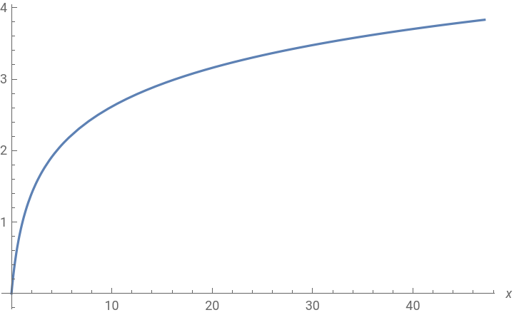
Next we look at the limits of the integral as x∞
Next we look at the limits of the integral as x∞