Stripping a Hydrocarbon from Oil Using Live Steam
Authors: Housam Binous and Ahmed Bellagi
Stripping a Hydrocarbon from Oil Using Live Steam
Authors: Housam Binous and Ahmed Bellagi
Authors: Housam Binous and Ahmed Bellagi
An oil containing 2.25 mole % of a hydrocarbon is stripped with live steam. Assume that 4 kmol of steam are used per 100 kmol of oil stripped.
The vapor-liquid relation of the hydrocarbon in the oil is=33.
Assume an isothermal operation by using internal heating, so that steam does not condense in the stripping tower.
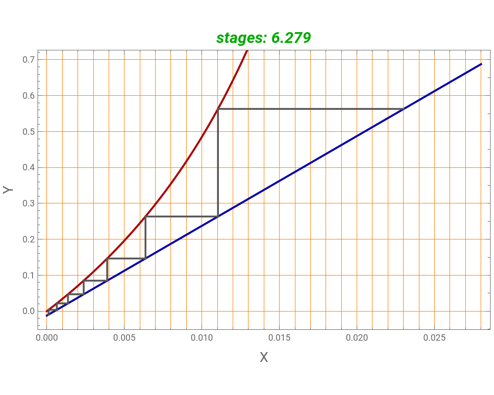
We plot the graphical construction (i.e., the operating line in blue and the equilibrium curve in red).
The staircase construction, shown in gray, gives the number of theoretical stages need to achieve the specified percent recovery of the hydrocarbon (assumed here to be equal to 97.8 %).
References :
1- J. M. Coulson, J. F. Richardson, J. R. Backhurst, and J. H. Harker, Coulson and Richardson’s Chemical Engineering: Solutions to the Problems in Volume 2 & 3, 2nd ed., Oxford: Butterworth–Heinemann, 1997.
The vapor-liquid relation of the hydrocarbon in the oil is
y
e
x
e
Assume an isothermal operation by using internal heating, so that steam does not condense in the stripping tower.
We plot the graphical construction (i.e., the operating line in blue and the equilibrium curve in red).
The staircase construction, shown in gray, gives the number of theoretical stages need to achieve the specified percent recovery of the hydrocarbon (assumed here to be equal to 97.8 %).
References :
1- J. M. Coulson, J. F. Richardson, J. R. Backhurst, and J. H. Harker, Coulson and Richardson’s Chemical Engineering: Solutions to the Problems in Volume 2 & 3, 2nd ed., Oxford: Butterworth–Heinemann, 1997.
Deriving the vapor-liquid relation in term of mole ratios labelled X and Y.
First, we find the mole fractions in term of mole ratios then we substitute these expressions in the equation:=33.
First, we find the mole fractions in term of mole ratios then we substitute these expressions in the equation:
y
e
x
e
In[]:=
Solve[Xx/(1-x),x]
Out[]=
x
X
1+X
In[]:=
Solve[Yy/(1-y),y]
Out[]=
y
Y
1+Y
In[]:=
Solve33,Y//FullSimplify
X
1+X
Y
1+Y
Out[]=
Y
33X
1-32X
In[]:=
eq[X_]:=33X/(1-32X);
plotting the equilibrium curve in red
In[]:=
plt1=Plot[eq[X],{X,0,0.015},PlotStyle{Thick,Darker@Red},FrameTrue,FrameLabel{Style["X",Italic],Style["Y",Italic]},GridLinesStyleDirective[Orange],ImageSize{500,400},GridLines{Table[i,{i,0,0.02,0.001}],Table[i,{i,0,0.9,0.1}]}];
The percent recovery of the hydrocarbon is assumed equal to 97.8 %.
2.25 is the inlet hydrocarbon concentration in the oil. Thus, the exit mole fraction of hydrocarbon in oil is 0.0495.
2.25 is the inlet hydrocarbon concentration in the oil. Thus, the exit mole fraction of hydrocarbon in oil is 0.0495.
In[]:=
percent=97.8;
In[]:=
sol=Solve[percent(2.25-xNP1)/2.25100,xNP1];
xNP1/.sol//First(*exitmolefractionofhydrocarbonintheoil*)
Out[]=
0.0495
XNP1=(xNP1/100/.sol)/(1-(xNP1/100/.sol))//First(*exitmoleratioofhydrocarbonintheoil*)
Out[]=
0.000495245
equation of the operating line
In[]:=
opt[X_]:=25X-25XNP1;
stepping off stages
In[]:=
i=1;X[1]=0.0225/(1-0.0225);(*inletmoleratioofhydrocarboninoil*)Y[1]=opt[X[1]];
In[]:=
While[X[i]≥XNP1,{X[i+1]=t/.FindRoot[eq[t]Y[i],{t,0.01}],Y[i+1]=opt[X[i+1]],Print[i," ",X[i+1]," ",Y[i+1]],i++}];
1 0.0110366 0.263534
2 0.00636047 0.146631
3 0.00389021 0.0848742
4 0.00237636 0.047028
5 0.00136294 0.0216923
6 0.0006438 0.00371386
7 0.000112137 -0.00957769
In[]:=
imax=i-1
Out[]=
7
In[]:=
fraction=((XNP1)-X[imax+1])/(X[imax]-X[imax+1])(*fractionofstage*)
Out[]=
0.720585
plotting the operating line in blue
In[]:=
plt2=Plot[opt[X],{X,0,0.028},PlotStyle{Thick,Darker@Blue},FrameTrue,FrameLabel{Style["X",Italic],Style["Y",Italic]},GridLinesStyleDirective[Orange],ImageSize{500,400},GridLines{Table[i,{i,0,0.028,0.001}],Table[i,{i,0,0.9,0.1}]},PlotLabelStyle["stages: "<>ToString[SetPrecision[imax-fraction,4]],Italic,Bold,16,Darker@Green]];
McCabe & Thiele diagram - We find that the number of stages required to achieve 97.8 % recovery is 7.
In[]:=
Show[plt2,plt1,Graphics[{Darker@Gray,Thickness[0.004],Table[Line[{{X[i],Y[i]},{X[i+1],Y[i]}}],{i,1,imax}],Table[Line[{{X[i],Y[i-1]},{X[i],Y[i]}}],{i,2,imax+1}]}],FrameLabel{Style["X",14],Style["Y",14]}]
Out[]=