The evolution of discrete systems can be difficult to predict, e.g. while cellular automata with periodic evolution can be accurately predicted with an autoencoder neural network, aperiodic, chaotic cellular automata generally cannot be predicted with much success. This study extends those ideas to another kind of discrete system, namely graph rewriting. In this work, a transformer neural network was trained on periodic and aperiodic graph rewriting systems to predict the next (or previous) step in their evolution, and to iteratively predict the entire forwards (or backwards) evolution of the system by using the previous prediction as the basis for the next. For undirected graphs whose node counts are conserved across their evolution, a simple transformer was able to predict the bidirectional evolution of a periodic case with perfect accuracy, but prediction of an aperiodic case had almost no success, comporting with previous findings for cellular automata; neural networks have only limited success in approximating graph rewriting rules as a function which maps the graph at state n to the graph at state n+1. These findings may suggest more broadly that artificial intelligences based on such current neural networks architectures as autoencoders and transformers are generally limited only to tasks also capable by humans (e.g., predicting the next step in a sequence that is easy to predict), doing so by tapping into the same pockets of computational reducibility accessible to human brains, but not tasks completely beyond human capability.
Introduction
Introduction
One of the uses of science is to predict what will happen next for a given system. The challenges associated with accurate prediction can be viewed as a manifestation of computational irreducibility [1], which in practice means that for many systems, the outcome of a process cannot easily be determined ‘ahead of time’; in many cases, the only way to find a later state of the system is to compute each step of the process along the way, from a given initial state at the initial step or ‘time’ to the desired number of steps or later ‘time’ (a kind of brute force approach). Prediction can be successful when, for a given system, a ‘pocket’ or ‘tunnel’ of computational reducibility [2] can be found, which can enable a process to be described mathematically, ideally by some closed-form solution [3]. (Though not necessarily a simple one!)Graph rewriting systems, which form the basis of the Wolfram Physics Project [4], are, in general, examples of computationally irreducible processes. For a given graph (that is, nodes connected by edges/relations) with a given rewriting/updating ‘rule’ (that is, the thing that tells the graph what to do next at each step/rewrite/update), it is generally very difficult to say what the graph will look like in the ‘future’ after a given number of steps/rewrites/updates without actually computing each step along the way (with the exception of the simplest possible cases). This is because in the world of computation, even simple rules can result in arbitrarily complicated behaviours or patterns, e.g. Rule 30 in elementary cellular automata [5].The aim of this project is to determine whether and which graph rewriting systems may contain pockets of computational reducibility that allow one to ‘jump’ forwards (or backwards) in the sequence of graph states, so as predict what will happen in ‘future’ (or, what has happened in the ‘past’) without having to explicitly compute all of the steps in-between. It may be that machine learning methods, including neural networks, can obtain a ‘general idea’ about how a given graph rewriting system works (i.e., to learn its rule) in such a way as to enable accurate prediction. In essence, the neural network has to learn the rule by approximating the function: which maps the graph at state n to the graph at state n+1 (i.e., the next step), with weights w fitted during training by minimizing a loss function (which describes the difference between the actual and predicted states). This might only be an example of ‘pattern matching’ rather than emergent science [6] – but might in any case have interesting applications e.g. in the Wolfram Physics Project, where studying the evolution of hypergraphs (e.g. to study a model universe’s exponent of growth or ‘effective dimensionality of space’) can be computationally intensive.Prior to this project, Wolfram [7] showed that an appropriate autoencoder neural network can predict the evolution of some simple cellular automata with some success, namely those whose evolution becomes repetitive or periodic. However, cellular automata with aperiodic, chaotic behaviour (a manifestation of computational irreducibility) are much more difficult for neural nets to learn from. Unsurprisingly, we show in this work that the same is true for graph rewriting.
f
w
S
n
S
n+1
Case 1: Periodic Graph Evolution
Case 1: Periodic Graph Evolution
Data
Data
For simplicity, in the following we consider only undirected graphs (for which each edge connects only two nodes [or a node to itself], and for which the adjacency matrices are symmetric along the main diagonal) and not directed graphs (for which the adjacency matrices are not necessarily symmetric) or hypergraphs (for which each [hyper]edge can connect more than two nodes). We also consider only rules that preserve the node count, i.e., graph rewriting systems that do not grow (or diminish) by adding (or removing) nodes. In a sense, this gives the neural net the best possible chance at accurate prediction.
The first N=1,000 updates of a simple graph rewriting system described by the rule {{a, b}, {b, c}, {c, d}} {{b, c}, {c, d}, {d, a}} and the initial state {{1, 2}, {2, 3}, {3, 4}} are computed to train the model. The evolution of the graph is animated in graph form (left below) and as corresponding adjacency matrices (right below), which indicate which nodes are connected.
The first N=1,000 updates of a simple graph rewriting system described by the rule {{a, b}, {b, c}, {c, d}} {{b, c}, {c, d}, {d, a}} and the initial state {{1, 2}, {2, 3}, {3, 4}} are computed to train the model. The evolution of the graph is animated in graph form (left below) and as corresponding adjacency matrices (right below), which indicate which nodes are connected.
Out[]=
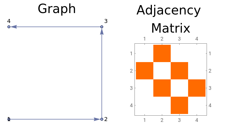
Evidently the system is periodic with a period of four (the same state [graph or adjacency matrix] appears again after every four rewrites/updates).
Modelling: Neural Network Classifier
Modelling: Neural Network Classifier
The simplest possible approach to modelling these data for prediction is to train a classifier with a neural network architecture, e.g. the model below, which is trained directly on the adjacency matrices for the first 1,000 steps using a dataset that relates each step n (the input) to the step n+1 (the desired output). A training:validation split of 80:20 is used, and the training data are shuffled.
Out[]=

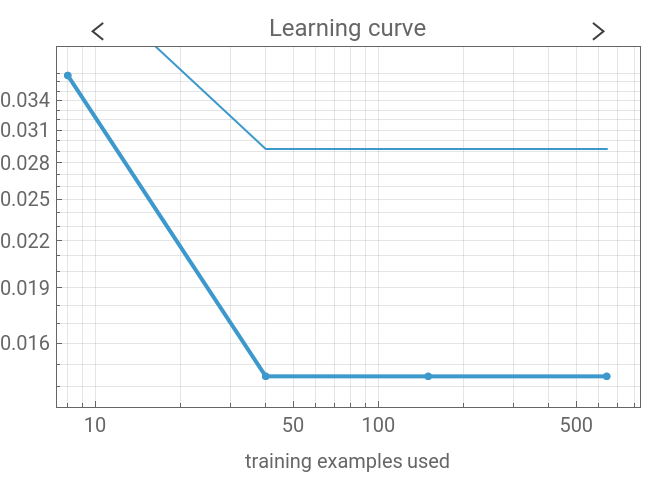
This approach is effective in terms of accuracy (>99%), but the use of a classifier is ‘cheating’ in a sense because it assumes the auxiliary hypothesis that the system has a finite number of states (classes). Thus, the classifier is simply matching like-to-like rather than ‘truly’ learning the rewriting rule as the function: .
f
w
S
n
S
n+1
Modelling: Transformer Neural Network
Modelling: Transformer Neural Network
In an attempt to really learn the rule, a transformer neural network is considered based on the architecture of the Generative Pre-Trained Transformer (GPT) model in the Wolfram Neural Net Repository [8], which is imported for reference below.
In[]:=
gptnet=NetModel["GPT Transformer Trained on BookCorpus Data"]
Out[]=
NetChain


The GPT transformer consists of encoder (called “embedding” in the imported model) and decoder modules. The encoder module converts raw input sequences into tokens (chunks of input) and maps (embeds) these into feature vectors, which represent some meaningful quality of the input. Tokens with similar positions in the feature vector space have similar meaning. The decoder layer uses attention mechanisms to self-direct attention to the most crucial tokens. Taken together, the encoder-decoder architecture of this net can be trained on input-output sequences to learn something about their structure and to produce the desired output (predictions).
In the case of the periodic graph rewriting system above, each graph state can be represented as a list of lists, where the inner lists represent pairs of connected/related nodes. E.g., {1,2} means that nodes 1 and 2 are connected/related. Rather than using the adjacency matrices as in the classifier above, the data used to train the transformer are in what is referred to here as ‘graph form’, e.g. the initial state in graph form is {{1, 2}, {2, 3}, {3, 4}}.
To prepare this into a sequence that the transformer can understand, each graph state (list of lists) is flattened with a delimiter separating each node pair, e.g. using the number 100 as a delimiter (the choice of delimiter number is arbitrary, as long as it never appears as a node in the graph; in this case, there are only 10 nodes, so a delimiter of 100 is appropriate [there is never a hundredth node]). E.g., the initial state in flattened, delimited form is {1, 2, 100, 2, 3, 100, 3, 4}.
The flattened, delimited sequences (graph states) are used to construct another dataset where each state is associated with the subsequent state (as in the dataset that was used for the classifier above, albeit with flattened, delimited graph states rather than adjacency matrices). The same 80:20 split is applied.
With this data format in mind, a new transformer model is constructed specific to these data. The encoder module of the GPT model in the Wolfram Neural Net Repository is extracted for reference below.
Out[]=
NetGraph

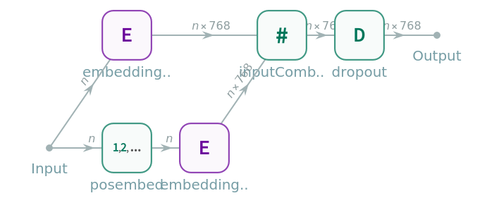

A similar encoder is (re)constructed from scratch, where the DropoutLayer (‘dropout’) specific to gptnet is excluded.
A similar encoder is (re)constructed from scratch, where the DropoutLayer (‘dropout’) specific to gptnet is excluded.
Out[]=
NetGraph

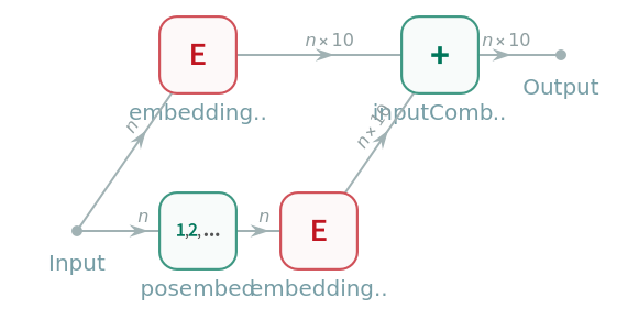
The diagram above shows that the input to this encoder module, which is a vector (list) of integers from 1 to 100 (as in the flattened, delimited graph states described above), undergoes two embeddings (one for capturing semantic meaning [tokens], the other for capturing positional meaning). These two embeddings are then combined (added together) to produce an output matrix consisting of 10 numbers (weights) for each of the elements of the input list.
With the encoder module set up, the decoder module can be constructed. The decoder module from the GPT model in the Wolfram Neural Net Repository is extracted for reference below.
With the encoder module set up, the decoder module can be constructed. The decoder module from the GPT model in the Wolfram Neural Net Repository is extracted for reference below.
Out[]=
NetChain
A similar attention head to that in the GPT model is (re)constructed from scratch, where the scaling ElementWiseLayer specific to gptnet is excluded.
A similar attention head to that in the GPT model is (re)constructed from scratch, where the scaling ElementWiseLayer specific to gptnet is excluded.
The attention mechanism above operates by taking each token, querying all others for contextual information, and responding to these queries with keys and values which provide the necessary contextual information. This mechanism therefore informs the network about the relative importance of each token, i.e., which tokens the network’s attention should be focused on to accurately capture the nature of the data.
The decoder module for the transformer is set up using 10 attention heads.
Finally, the encoder and decoder modules set up above are combined into a transformer.
The transformer above operates by:
1. Encoding/embedding the input data to capture contextual/positional information.
2. Decoding the encoded/embedded input to focus the network’s attention with attention mechanisms.
(Steps 1 and 2 above identify important patterns in the input data.)
3. Encoding/embedding the target data using the same weights as the encoder for the input data to capture (ideally) the same contextual/positional information there.
4. Computing the loss between the processed input data and processed target data (loss 1).
(Steps 3 and 4 above map the input data to the target data.)
5. Computing the loss between the encoded/embedded and subsequently processed target data and the original target data (loss 2).
6. Computing the total loss (loss 1 + loss 2), which is minimized during training to get the desired output from the input.
With the transformer defined, it is trained on the flattened, delimited graph data.
The loss curve above suggests that the model has learned from the data.
Lastly, the trained net is used to make predictions about the next step in the graph evolution. To do so, the trained net is used to generate a prediction for step #2 based on the actual step #1, then this prediction is fed back into the transformer to predict step #3, then this prediction is fed back into the transformer to predict step #4, and this iterative process is repeated to predict the entire future evolution of the system.
Lastly, the trained net is used to make predictions about the next step in the graph evolution. To do so, the trained net is used to generate a prediction for step #2 based on the actual step #1, then this prediction is fed back into the transformer to predict step #3, then this prediction is fed back into the transformer to predict step #4, and this iterative process is repeated to predict the entire future evolution of the system.
Finally, it is possible to do the same in reverse, i.e. to start with some given ‘future’ state and work backwards to recover the initial condition. To do this, it is necessary to retrain the net with the associations between states reversed.
Finally, it is possible to do the same in reverse, i.e. to start with some given ‘future’ state and work backwards to recover the initial condition. To do this, it is necessary to retrain the net with the associations between states reversed.
So, the transformer neural net can predict the past and future of a simple periodic graph rewriting system. Next, a more complicated system giving rise to aperiodic behaviour is considered to determine the extent to which neural nets are ‘blocked’ by computational irreducibility in graph rewriting.
So, the transformer neural net can predict the past and future of a simple periodic graph rewriting system. Next, a more complicated system giving rise to aperiodic behaviour is considered to determine the extent to which neural nets are ‘blocked’ by computational irreducibility in graph rewriting.
Case 2: Aperiodic Graph Evolution
Case 2: Aperiodic Graph Evolution
Data
Data
In this case, a graph whose evolution is not periodic (at least for the period of its evolution under consideration) is considered. Many aperiodic graphs grow in node/edge count, with the growth described as linear, exponential, or other [9]. Growing graphs quickly require large quantities of memory to store. Thus, for simplicity, this case considers a graph that is aperiodic and whose node count is conserved so that nodes are neither created nor destroyed.
The first N=100,000 updates of an aperiodic updating graph described by the rule {{a, b}, {b, c}, {c, d}} {{c, d}, {d, b}, {b, a}} and initial state {{1, 2}, {2, 3}, {3, 4}, {4, 5}, {5, 6}, {6, 7}, {7, 8}, {8, 9}, {9, 10}, {10, 1}, {9, 2}} are computed. Since running 100,000 updates on this graph is too computationally intensive for the machine this notebook was prepared on, the Wolfram Remote Batch (cloud computation) was used, taking ~14 hours and costing 714 Wolfram Service Credits.
The first few graph/adjacency matrix states for this system are animated below.
From the animations above, the graph appears to produce updates that are aperiodic and difficult to predict by eye, despite consistently applying the same simple rule. This behaviour is unlike the previous periodic case, which was intuitive and easy to predict.
Upon closer inspection, it actually appears that this rule is not truly aperiodic:
In other words, it is aperiodic for the first 727 states, but then settles into a periodic system with period 84,952, starting with the 728th state. In order for the model to actually learn the rule rather than simply ‘cheating’ by noticing this long-term periodicity in the training data, the model is trained on only the first 85,678 states.
Modelling: Transformer Neural Network
Modelling: Transformer Neural Network
The same transformer neural network defined above, which was successful in predicting the periodic case, is re-trained for the aperiodic case with data from the aperiodic system.
Again the loss curve suggests something is learned.
Finally, the re-trained net can be used to make predictions about the next step in the aperiodic graph evolution. The predictions seem somewhat reasonable when predicting each next single step using each known, previous step (i.e., without feeding each prediction back into the model iteratively)...
Finally, the re-trained net can be used to make predictions about the next step in the aperiodic graph evolution. The predictions seem somewhat reasonable when predicting each next single step using each known, previous step (i.e., without feeding each prediction back into the model iteratively)...
... But iterative prediction (i.e., feeding each prediction back into the model to predict the entire future sequence from the initial state) fails after the first few states as errors are compounded, and the predicted system quickly becomes periodic.
Similarly, the actual graph predictions are completely inaccurate.
Concluding Remarks
Concluding Remarks
This project explored the use of neural networks to predict graph rewriting systems. While the transformer neural network model in this work can predict the forwards and backwards evolution of a periodic graph rewriting system with perfect accuracy, it has only very limited success in predicting the next single step of an aperiodic graph rewriting system, and no success at all in predicting the long-term evolution of an aperiodic system. These findings comport with Wolfram’s [6] modelling of cellular automata evolution, namely that periodic cellular automata can be predicted by autoencoder neural networks while aperiodic cellular automata cannot. This result is not terribly surprising, as this is essentially equivalent to saying that easy-to-predict discrete systems are easy to predict, while difficult-to-predict discrete systems are difficult to predict. Nevertheless, these findings may have implications for such broad claims that artificial intelligences, at least those based on such neural networks architectures as autoencoders and transformers, are unlikely to be able to one day ‘do anything’; where there is computational irreducibility, as there is in aperiodic discrete systems, models will struggle.
There are a number of potential avenues for future works in this area. First and foremost, the particular neural network architecture implemented in this work is unlikely to be the best possible model, since it was originally designed for text. In particular, the way tokenization occurs is likely to impact the predictive performance of the model significantly. There exist so-called ‘graph transformer’ models with novel graph structural encodings (see e.g. the ‘graphormer’ [10]) which are likely more appropriate. Attention can be applied to each node to better capture qualities of the graph structure. In addition to other models, more graphs could also be considered; not only is it possible (though computationally intensive) to produce more training data and therefore potentially improve predictive performance, more fundamentally this study considered only those graphs whose edges were undirected and connected two nodes, while directed graphs and hypergraphs could also be considered. Furthermore, this work only considered graph rewriting systems whose node counts were constant; future works could consider systems that grow (or diminish) in edge count [9], though the memory requirements for studying such systems are high.
Another point to consider is that in the kinds of graph rewriting systems relevant to the Wolfram Physics Project [4], there is more than one ‘path of time’, because there are many ways to apply the same rule, potentially resulting in very different-looking rewrites. This presents an additional level of complexity for neural networks trained to approximate graph rewriting systems; they have to learn not only the rule, but also the way or order in which it is being applied to produce each new hypergraph. Future works may therefore seek to apply neural networks to multiway graphs [11] and branchial graphs [12] to capture some of this additional complexity.
A final point to consider is whether even successful prediction of graph evolution by neural networks can really be considered an example of computational reducibility; if the computational requirements of generating sufficient training data and then training a given model to predict n additional steps ahead actually meets or exceeds the computational requirements of simply computing those n steps directly, then the pocket of computational reducibility the net has seemingly tapped into might more accurately be described as a false pocket (i.e., a detour rather than a shortcut). If neural nets can only access the same pockets of computational reducibility accessible to a human brain (e.g. the easily-predicted periodic system explored in Case 1 above), then their utility in this regard is limited. Still, if the purpose is to learn something fundamental about the system (e.g. when the rule is actually unknown) rather than simply to make predictions about what will happen next, then modelling discrete systems with neural nets may still have some utility.
Acknowledgements
Acknowledgements
References
References
1. Rowland, Todd. “Computational Irreducibility.” From MathWorld--A Wolfram Resource, created by Eric W. Weisstein. https://mathworld.wolfram.com/ComputationalIrreducibility.html
2. Rowland, Todd. “Computational Reducibility.” From MathWorld--A Wolfram Resource, created by Eric W. Weisstein. https://mathworld.wolfram.com/ComputationalReducibility.html
3. Weisstein, Eric W. “Analytic.” From MathWorld--A Wolfram Resource. https://mathworld.wolfram.com/Analytic.html
4. Wolfram, Stephen. 2020. A Project to Find the Fundamental Theory of Physics. Wolfram Media, Inc. https://wolframphysics.org/
5. Weisstein, Eric W. “Rule 30.” From MathWorld--A Wolfram Resource. https://mathworld.wolfram.com/Rule30.html
6. Wolfram, Stephen. 2024. Stephen Wolfram: Can AI Solve Science? https://www.youtube.com/watch?v=goYaSkxG8LA&t=1427s
7. Wolfram, Stephen. 2024. “Can AI Solve Science?” Stephen Wolfram Writings. https://writings.stephenwolfram.com/2024/03/can-ai-solve-science
8. Wolfram Neural Net Repository. 2019. GPT Transformer Trained on BookCorpus Data. https://resources.wolframcloud.com/NeuralNetRepository/resources/GPT-Transformer-Trained-on-BookCorpus-Data
9. Kansal, Jatin. 2020. Classify growth rates for Wolfram Models. https://community.wolfram.com/groups/-/m/t/2028496
10. Ying, Chengxuan et al. 2021. Do Transformers Really Perform Bad for Graph Representation? https://doi.org/10.48550/arXiv.2106.05234
11. Weisstein, Eric W. “Multiway Graph.” From MathWorld--A Wolfram Resource. https://mathworld.wolfram.com/MultiwayGraph.html
12. Weisstein, Eric W. “Branchial Graph.” From MathWorld--A Wolfram Resource. https://mathworld.wolfram.com/BranchialGraph.html
Cite This Notebook
Cite This Notebook
Mining Pockets of Computational Reducibility with AI: Transformer Models of Graph Rewriting
by Floe Foxon
Wolfram Community, STAFF PICKS, July 9, 2025
https://community.wolfram.com/groups/-/m/t/3495324
by Floe Foxon
Wolfram Community, STAFF PICKS, July 9, 2025
https://community.wolfram.com/groups/-/m/t/3495324