Abstract: The project is concerned with discovering correlations between the growth of dimensionality of the model with the number of steps applied. The first step is to categorize the rules based on whether they lead to increasing, decreasing or periodic relationships with the number of dimensions. Based on that information, it may be possible to study the connection to particle physics - to explore how the de Sitter entropy of the universe relates to the entropy of the graph. The results will also be relevant to study the correspondence between the evolution of the Wolfram models and early universe inflation models - to analyze the evolution of the quantum degrees of freedom as the universe was expanding.
Main findings: classification of the rules based on the value of the slopes of their dimensionality graph approximations; alternative approach to dimensionality approximation, distributions of the universes based on their stability.
Next steps: Exploring other signatures, getting a larger set of results for the initial condition variance for the spectral dimension.
Motivation,GoalandBackground
The notion of dimension is crucial for characterizing the limiting behaviors of the models, especially when the traditional geometrical structures of the graphs are not readily recognizable. The progression of dimensionality with an increased number of steps can tell us two things about a universe that is being studied. First, whether it is static, contracting, or expanding. And second, we get a better idea about the behavior of the universe at its boundary effects. Usually, to approximate the dimensionality of the graph, we look at the Hausdorff dimension and calculate the log difference between the neighborhood hypervolume values. Essentially, we approximate d in the scaling law V = , where V is the volume of a graph, and r is the distance from the central node to its neighbors. The question is, what happens to the volume when d is a function of time, i.e., the number of evolutions. A solution proposed in this project is to use the values the the neighborhood volume to fit a linear regression, record the slope, and classify the rules based on those results. The slope is then in units of dimensions. However, we also find that this type of dimensionality approximation is not efficient. First, it is sensitive to boundary effects, and thus can be not representative of the true dimensionality of the universe in that part of the range. We propose an alternative approach using the spectral dimension. We find an average length of a random walk starting from the most connected node, and use those values to learn about the correlation with the number of evolutions. We have to set some constraints onto the signatures and the states of the graph. The project is only implemented for signatures and only for connected hypergraphs. The caveat of the disconnected case is in the definition of dimension - one would need to decide whether only to consider the largest connected component or something alternative.
d
r
2
2
3
2
Variable
There are three variables that we can vary:
- the initial conditions of the hypergraphs based on the signature;
- the update rules based on the signature;
- the way that the rules are applied, i.e. least recent edge/random.
Here,we only work with the first two, i.e.explore the variation with the initial conditions as well as the variation with different rules.
Let’s begin with a demonstration of the approach on the classic example.
Example
Example
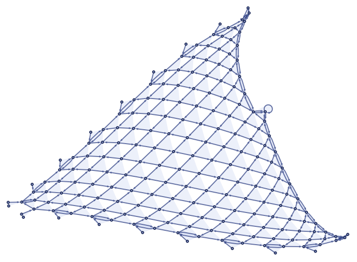
Let'sconsiderasimplegridcorrespondingtoarule
2
2
3
3
In[]:=
eo = WolframModel[{{1, 2, 2}, {3, 1, 4}} -> {{2, 5, 2}, {2, 3, 5}, {4, 5, 5}}, {{0, 0, 0}, {0, 0, 0}}, 200]; eo["FinalStatePlot"]
Out[]=
Hausdorffdimension
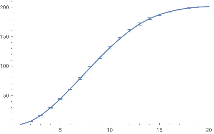
Now, let' s have a look at a Hausdorff dimension approximation.
In[]:=
ListLinePlot[ResourceFunction["RaggedMeanAround"][Values[ResourceFunction["HypergraphNeighborhoodVolumes"][eo["FinalState"]]]]]
Out[]=
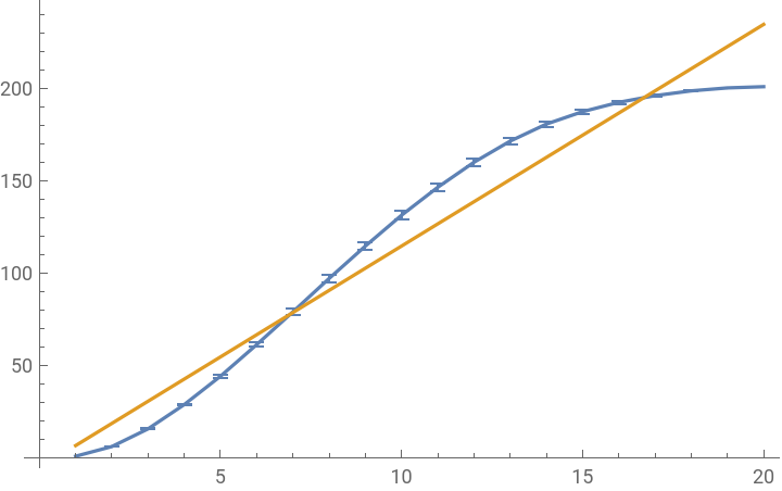
The code below fits the linear regression to the curve and outputs the slope.
In[]:=
rma = ResourceFunction["RaggedMeanAround"][Values[ResourceFunction["HypergraphNeighborhoodVolumes"][eo["FinalState"]]]];p=Predict[Range[Length[rma]] rma,Method"LinearRegression"];pred = p[Range[Length[rma]]];slope = (pred[[-1]] - pred[[1]])/Length[pred];gr = List[rma, pred]; Show[ListLinePlot[Table[gr[[i]], {i, 1, Length[gr]}]]]
Out[]=
Spectraldimension
Below is the code for the spectral dimension approximation. We run a random walk using thee adjacency matrix as a set of the update rules. Essentially, it is a Markov chain with a uniform probability distribution for each node that is connected to the starting node.
In[]:=
getTrMatrix [gr_] := Module[{},adj = Normal[AdjacencyMatrix[gr]];adjTr = adj + Transpose[adj];adjNorm = Table[adjTr[[i]] / (adjTr[[i]] // Total), {i, 1, Length[adjTr]}]; adjNorm]
Then, we randomly select the next step and update the current position. We proceed until we get back at the starting point.
In[]:=
randWalkStep[i_, matrix_] := Module[{}, elements = Range[Length[matrix]];probs = matrix[[i]];sample = RandomChoice[probs elements];sample]randWalk[matrix_,start_]:= Module[{},current = start; walk = List[];count = 0 ;If[Length[matrix] 1, AppendTo[walk, 0]; Print["zero dim"]; Break[], While [True, sample = randWalkStep[current, matrix]; count ++; If[sample == start, AppendTo[walk, count]; Break[], current=sample]]];walk];
We define the starting point as the central and most connected node.
In[]:=
randWalkGraph[state_]:= Module[{}, gr = ResourceFunction["HypergraphToGraph"][state];center = Part[VertexList[IndexGraph[gr]],Ordering[RadialityCentrality[gr],All,Greater]][[1]];adjM = getTrMatrix [gr];If[Length[adjM] > 1, res = Flatten[Table[randWalk[getTrMatrix [gr] , center], {i, 1,1000}]];Round[Mean[res]], 0]]
Here is the result of the spectral dimension approximation for the example graph.
In[]:=
fs = ResourceFunction["WolframModel"][{{1,2,2},{3,1,4}}{{2,5,2},{2,3,5},{4,5,5}},{{0,0,0},{0,0,0}},200, "StatesList"];ListLinePlot[ParallelTable[randWalkGraph[fs[[i]]], {i, 1, Length[fs]}]]
Out[]=
As we can already see, we get less sensitive to the boundary conditions.
Results
For the chosen signature, we have eight initial conditions.
In[]:=
initStates={{{0,0},{0,0}},{{0,1},{1,0}},{{0,1},{1,2}},{{0,1},{0,2}},{{0,0},{0,1}},{{0,1},{0,1}},{{0,1},{2,1}},{{0,0},{1,0}}};buildGraph[state_] := Graph[Table[state[[i]][[1]] state[[i]][[2]], {i, 1, Length[state]}]]; Table[buildGraph[initStates[[i]]], {i, 1, Length[initStates]}]
The histograms above show the distribution of the slope values for the initial condition values. We selected all of the rules that lead to connected hypergraphs. As we can see, the majority of the the rules have dimensionality curves with zero slopes, which indicate stable universes.
For the spectral dimension the results are the following.
There are much less samples in this case due to computational complexity. We can see that for some conditions, we are getting negative slopes. That is an indicator of contracting universes.
A huge thanks to Jack Heimrath and Jonathan Gorard, who were wonderful and supportive mentors throughout the project. Also to Kiel Howe - a professor at Minerva Schools who provided theoretical and practical preparation for the physics track. Additionally, I thank Stephen Wolfram and the Summer School organizers for a remarkable opportunity to participate in this project.