A computational reading of Aaron J. Miller, Sae Woo Nam, John M. Martinis, Alexander V. Sergienko; Demonstration of a low-noise near-infrared photon counter with multiphoton discrimination. Appl. Phys. Lett. 28 July 2003; 83 (4): 791–793. https://doi.org/10.1063/1.1596723
A monochromatic light pulse can deposit only a discrete set of energies in an absorber: , , , , and so on. This is the most basic statement of the quantization of the electromagnetic field. The 2003 paper turns it from a textbook statement into a direct picture. A weak laser pulse hits a tungsten transition-edge sensor (TES) 120,000 times. The TES measures the total energy deposited by each pulse. The histogram of those energies (Figure 2 of the paper) shows distinct peaks at integer multiples of , with nothing in between. Each peak is the Fock state (a definite-photon-number eigenstate) of the field showing up as a measurable quantity of heat.
0
hν
2hν
3hν
hν
|n〉
Three pieces of physics combine to make that picture possible. The energy ladder =nhν is set by quantum electrodynamics. The relative populations of the rungs are set by the source: a coherent laser pulse populates them with Poisson weights. The peak widths are set by the detector: an irreducible thermodynamic noise floor =C, plus a small engineering excess. We compute each piece below, combine them as a mixture distribution, and reproduce the figure by Monte Carlo.
E
n
σ
E
k
B
2
T
Why I did this computation. This paper was one of the topics John Martinis presented at APS 2026 in his talk as a 2025 Nobel laureate. Two things caught my attention. The first was a physical point John emphasized: this experiment makes the quantization of light directly visible in the raw measurement, in a way that the Planck blackbody spectrum does not. Planck’s law was, of course, born from energy quantization, but the smooth thermal curve that comes out of it shows no obvious sign of “discrete photons” to a non-expert eye; the quantization sits in the derivation, not on the screen. Figure 2 of the 2003 paper, by contrast, is the quantization itself, plotted as separate peaks one photon apart. The second reason (more important to me) was personal. John told the story with visible excitement, eyes bright, and said he still remembers the moment he first saw those measurement dots line up on integer rungs and how thrilling that was. I wanted to understand the physics well enough, and concretely enough, that I could feel some fraction of that same excitement when watching a law of nature reveal itself in a histogram.
A note on which paper this notebook reproduces. The slide John showed cites the 1998 works by Cabrera and co-authors, the first proof that a tungsten TES microcalorimeter can resolve photon number, demonstrated across several wavelengths. The notebook here reproduces the natural follow-up: the 2003 paper by Miller, Nam, Martinis and Sergienko, refined at the 1550 nm telecom wavelength with the full Poisson-times-Gaussian fit and the dark-count and noise-equivalent-power numbers that frame the device for use in quantum key distribution.
A calorimeter to read the photons
A calorimeter to read the photons
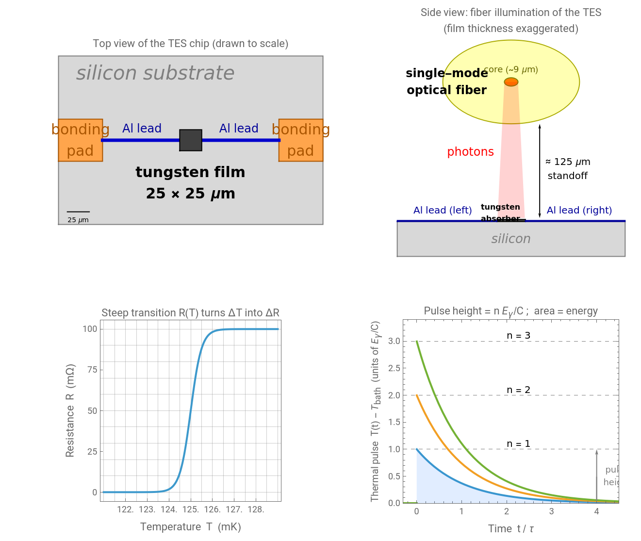
An avalanche photodiode tells you only that something hit it; the avalanche saturates and erases photon-number information. A calorimeter is different: it measures total deposited heat, so its output really is proportional to . The TES of this paper achieves that with a thin tungsten film — m × m × 35 nm on silicon — biased on the very steep edge of its superconducting transition at ∼125 mK, where the resistance changes by tens of m over a transition width mK. A small absorbed energy raises the temperature; the resistance jumps along the steep edge; the integrated current pulse is proportional to the deposited energy. Aluminum leads, also superconducting at this temperature, are thermally insulating enough to keep the heat localized in the tungsten long enough to read out.
n
E
γ
25μ
25μ
T
c
Ω
Δ∼1
T
c
The below four-panel composite shows the entire physics chain that turns a single near-infrared photon into a measurable count, all on one chip. Top left is the chip seen from above: a 25 μm × 25 μm tungsten film (dark square) at the center of a millimeter-scale silicon substrate, contacted by two superconducting aluminum traces that run out to bonding pads — the tungsten is both the photon absorber and the thermometer. Top right is the same chip seen edge-on, with a single-mode optical fiber (~9 μm core) suspended ~125 μm above the absorber so its slightly diverging beam lands on the film through free space. Bottom left is the operating principle of the thermometer: tungsten’s resistance jumps from 0 to ~100 mΩ over a transition width of only ~1 mK at ≈125 mK, and the device is voltage-biased on the steepest part of that edge — a tiny temperature change from an absorbed photon therefore produces a large resistance change , which is the calorimeter’s gain. Bottom right is what comes out: each absorbed photon dumps energy into the absorber’s heat capacity , the temperature rises by for photons absorbed simultaneously, and the resulting thermal pulse decays back to the bath with time constant μs — the peak heights stack on a perfect integer ladder () and the integrated area equals the deposited energy. Read clockwise from top-left: photon arrives at the absorber, raises its temperature by sub-millikelvin amounts, the steep converts that into a measurable resistance step, and the resulting current pulse — integer-spaced in — fills the histogram peaks of Figure 2 of the paper.
T
c
ΔT
ΔR
E
γ
C
nC
E
γ
n
τ≈15
n=1,2,3,…
R(T)
n
Two timing facts are essential. The optical pulse is 100 ns wide; the detector relaxes over 15 s. The pulse is so short relative to the relaxation that all photons in one pulse are absorbed inside one thermal event — the detector cannot tell them apart in time, so it sums their energies. Pulses repeat at 500 Hz (every 2 ms), much longer than the relaxation, so adjacent events are independent. Both inequalities are required: the first turns photon counting into a single calorimetric measurement; the second turns the histogram into a sequence of independent draws.
μ
Out[]=
pulse width | |
detector fall time | |
repetition interval | |
fall / pulse | 150 |
interval / fall | 133.333 |
The thermodynamic resolution floor
The thermodynamic resolution floor
For a monochromatic source the only allowed amounts of deposited energy are integer multiples of one photon's worth, =hcλ. At the telecom wavelength nm:
E
γ
λ=1550
In[]:=
ePhoton=UnitConvert[Quantity["PlanckConstant"]*Quantity["SpeedOfLight"]/Quantity[1550,"Nanometers"],"Electronvolts"]//N
Out[]=
Why is the paper's =0.120 eV the right order of magnitude? Even with perfect electronics, a body of heat capacity in equilibrium with a bath at temperature has internal-energy variance =C — a textbook result of canonical-ensemble statistical mechanics. The paper says explicitly that dark counts are determined solely by the intrinsic 125 mK thermal fluctuations of the device, so this floor sets both the dark-count rate and the smallest detectable signal.
σ
E
C
T
2
σ
E
k
B
2
T
Build the heat capacity from the film geometry. Material constants come from ElementData so nothing is hardcoded:
In[]:=
filmArea=Quantity[25,"Micrometers"]Quantity[25,"Micrometers"];thickness=Quantity[35,"Nanometers"];volume=UnitConvert[filmArea*thickness,"CubicMeters"];
In[]:=
density=ElementData["Tungsten","Density"];molarMass=ElementData["Tungsten","MolarMass"];moles=(density*volume)/molarMass
Out[]=
The electronic specific heat of a normal metal is =γTN, with the Sommerfeld coefficient ≈1.3 mJ/(mol·K) for tungsten. On the superconducting transition Bardeen–Cooper–Schrieffer (BCS) theory predicts a jump /≃2.43, so use that:
C
e
γ
W
2
C
s
C
n
In[]:=
γSommerfeld=UnitConvert[Quantity[1.3,"Millijoules"/("Moles""Kelvins"^2)],"Joules"/("Moles""Kelvins"^2)];Tc=Quantity[125,"Millikelvins"];Cabsorber=UnitConvert[2.43γSommerfeld*Tc*moles,"Joules"/"Kelvins"]
Out[]=
Now plug into =C and convert to electronvolts. Use this derived value as the energy resolution from this point on — no hardcoded fit parameter:
σ
E
k
B
2
T
c
In[]:=
σE=UnitConvert[Sqrt[Quantity["BoltzmannConstant"]*Tc^2*Cabsorber],"Electronvolts"]
Out[]=
The paper's two-parameter fit to the data gave =0.120±0.017 eV — about 1.4× this floor. The excess comes from readout noise in the superconducting quantum interference device (SQUID) amplifier chain and electrothermal-feedback noise in the bias loop, neither of which is in our model. Our peaks will therefore be a bit narrower than Figure 2 (better separation), but the integer-rung structure and the Poisson populations are unchanged. The order of magnitude — tens of meV at this and absorber size — is not an engineering choice; it is fixed by thermodynamics.
σ
E
T
c
The figure of merit for resolving the ladder is the ratio of rung spacing to peak width :
E
γ
σ
E
In[]:=
""->ePhotonσE,"σ (photon units)"->σEePhoton
E
γ
σ
E
Out[]=
9.17475,σ (photon units)0.108995
E
γ
σ
E
About 9 (paper's measured value gives ~7). The rungs are well separated by either number. At shorter wavelength grows but does not, so the ratio grows — exactly the pattern the paper reports across 670, 830, 1310, 1550 nm.
E
γ
σ
E
Which rungs the source populates: coherent state Poisson
Which rungs the source populates: coherent state Poisson
Resolving the rungs is half the story; the heights of the peaks tell us about the source. A laser well above threshold produces a coherent state , defined as an eigenstate of the photon annihilation operator,
|α〉
a
with the Fock-basis expansion
|α〉=|n〉.
-α2
2
∞
∑
n=0
n
α
n!
The probability of measuring exactly photons is with =. Verify by symbolic algebra that this is the Poisson probability mass function (PMF) with mean :
n
|
c
n
2
c
n
-α2
2
n
α
n!
μ=|α
2
In[]:=
cCoeff[n_,α_]:=Exp[-Abs[α]^2/2]α^n/Sqrt[n!]
In[]:=
Simplify[Abs[cCoeff[n,α]]^2==PDF[PoissonDistribution[Abs[α]^2],n],Assumptions->{n>=0,n∈Integers,α∈Reals,α>0}]
Out[]=
True
True. Poisson statistics are not a model assumption but a direct consequence of the source being a coherent state. The paper's two-parameter fit to Figure 2 gives . This is the only experimental fit value we use; all other parameters in the analysis are derived. For that mean, the populated rungs cluster around –:
μ=4.02±0.16
n=3
4
μ=4.02;(*meanphotonnumberperpulse,frompaper'sfit*)DiscretePlotPDF[PoissonDistribution[μ],n],{n,0,15},
Out[]=
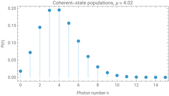
These are the relative weights the peaks of Figure 2 must have.
The full predicted spectrum
The full predicted spectrum
Reproducing Figure 2
Reproducing Figure 2
Every event has fallen on a rung — and the populations of the rungs follow the Poisson curve. The agreement is exact in this Monte Carlo because we drew from the same generative model the curve was built from. The next section asks the harder question: in the real experiment, are the deviations consistent with counting noise alone?
Concluding Remarks
Concluding Remarks
What the paper shows, and what we have rebuilt computationally above, is a single direct picture of the quantization of the electromagnetic field. A monochromatic light pulse cannot deposit a continuous range of energies into matter. It deposits energy only in integer multiples of one photon's worth, and a sufficiently sensitive heat-measuring device sees those multiples as separate, countable peaks. Earlier demonstrations of field quantization, such as photon antibunching from single-emitter sources or photoelectric thresholds, are about the absence of certain outcomes. This experiment is the positive statement: every absorption event is a definite number of photons, and the histogram of those numbers is the raw photographic record of the field's number-state structure.
Three pieces of physics had to come together in one chip to make the picture clean. The first is the calorimetric idea itself. By measuring total deposited heat instead of a triggered click, a TES converts photon counting into energy measurement, and energy is what the field quantizes. The second is the steep superconducting transition of the tungsten film. The transition turns a sub-millikelvin temperature step into a measurable resistance step, giving the calorimeter the gain it needs to read out single optical photons against the thermodynamic noise of the absorber. The third is the chain of cryogenics, low-noise amplification, and timing that makes the readout fast enough to register a single thermal event before it relaxes back to the bath.
The shape of the histogram tells two stories at once. The positions of its peaks are dictated by quantum electrodynamics: photons of a given wavelength carry a fixed energy, and integer numbers of them deposit integer multiples of that energy. The relative heights of the peaks are dictated by the source: a coherent laser pulse populates the photon-number ladder with the well-known Poisson distribution, and that envelope falls right on top of the integer rungs. Because the peak widths come from the detector and the peak positions and weights come from the field, a single calorimetric measurement separates source physics from detector physics in one image.
The same instrument that exhibits field quantization also acts as a metrology and security tool. Earlier photon-number techniques, such as the Hanbury Brown-Twiss correlation, can distinguish only between one photon and more than one, with limited efficiency, while a TES reads the full photon-number distribution in a single channel with negligible dark counts. That capability is what makes this device the right instrument for validating single-photon sources used in quantum key distribution: any leakage of multi-photon emission shows up directly in the histogram as a peak weight that is too large. The paper's reported dark-count and noise-equivalent-power figures translate that capability into a meaningful range advantage for fiber-based quantum cryptography. Energy quantization, made visible by a calorimeter, becomes a working tool.
CITE THIS NOTEBOOK
CITE THIS NOTEBOOK
Photographing the quantization of light
by Mohammad Bahrami
Wolfram Community, STAFF PICKS, May 1, 2026
https://community.wolfram.com/groups/-/m/t/3710411
by Mohammad Bahrami
Wolfram Community, STAFF PICKS, May 1, 2026
https://community.wolfram.com/groups/-/m/t/3710411