Examples for working with finite automata (deterministic, non-deterministic and epsilon)
by Tomás de Camino Beck
by Tomás de Camino Beck
Introduction
Introduction
I have created a series of posts regarding finite state machines. On this post, I just show several examples of using Mathematica to evaluate finite state automata, either deterministic, non deterministic, or non-deterministic with epsilon transitions.
Most of these examples are textbook examples, meant for teaching purposes.
Here I use just a few functions to compute strings over a state machine definition, determine if a string is valid, and then give you some functions for displaying the graph and the transition table.
Most examples are taken from Hopcroft & Ullman, or Sipser’s book.
Defining an Automata
Defining an Automata
For defining an automata we use associations. Each transition function is defines as an association , where a rule is defines as . Symbols are declared as characters (except for empty symbol ϵ). Look carefully at the examples to get a good idea on how to define automata transitions.
δ
,,…
key
1
val
1
key
2
val
2
keyval
{state,"symbol"}{stateorstates}
Basic Functions
Basic Functions
Finite Automata Computation
Finite Automata Computation
In[]:=
Closure[δ_,state_List]:=Union[Map[Flatten[Most[NestWhileList[Union@@Table[δ[{#1[[i]],ϵ}]/._Missing{},{i,Length[#1]}]&,{#},#≠{}&]/._Missing{}]]&,state]//Flatten]DeltaHat[δ_,q0_List,string_]:=FoldList[Closure[δ,Union@@Table[δ[{#1[[i]],#2}]/._MissingNothing,{i,Length[#1]}]]&,Closure[δ,q0],Characters[string]]IsValidQ[δ_,q0_List,qf_List,string_]:=ContainsAny[qf,Fold[Closure[δ,Union@@Table[δ[{#1[[i]],#2}]/._MissingNothing,{i,Length[#1]}]]&,Closure[δ,q0],Characters[string]]]
Usage
Usage
DeltaHat[association, {initial_state}, string]
Computes string using the transitions defined by association starting from initial_state. Returns the states reached for each character in string (from left to right)
IsValidQ[association, {initial_states}, {final_states},string]
Computes string using the transitions defined by association starting from initial_state. true or false if any of the final_states are reached
Graph Creation
Graph Creation
In[]:=
ShowGraphFA[edges_,states_List,q0_,q_List,edgelabels_,opts___]:=Graph[edges,VertexSize0.25,VertexLabelsPlaced["Name",Center],VertexStyleJoin[{0White},Map[(#Red)&,q]],EdgeWeightedgelabels,EdgeLabels"EdgeWeight",opts]
Usage
Usage
ShowGraphFA[edges, states,{ initial_states}, {final_states},{edge_labels}]
Shows a graph with directed edges. initial_states are drawn white, final_states are red. edge_labels have to be specified in the same order as the edges
Transition Table
Transition Table
In[]:=
FATable[δ_,states_,Σ_,opts___]:=Grid[Join[List/@Prepend[states,"Q\Σ"],Prepend[Partition[Flatten[Outer[δ[{#1,#2}]/._Missing"-"&,states,Σ,1],1],Length[Σ]],Σ],2],AlignmentCenter,Spacings{2,1},FrameAll,ItemStyle"Text",Background{{Gray,None},{LightGray,None}},opts]
Usage
Usage
FATable[association, states_list ,alphabet_list]
Creates a transition table for the automata defined with association, using the states_list, with symbols from the alphabet_list
Example 1
Example 1
Strings Accepted: This automata accepts (Example taken from Sipser’s book). Start state 0, final states {1,3}
{|nis even or divisible by3}
n
a
Definition:
In[]:=
δ=Association[{0,ϵ}{1,3},{1,"a"}{2},{2,"a"}{1},{3,"a"}{4},{4,"a"}{5},{5,"a"}{3}];
Graph :
In[]:=
ShowGraphFA[{01,03,12,21,34,45,53},{0,1,2,3,4,5},{0},{1,3},{"ϵ","ϵ","a","a","a","a","a"},ImageSize->Large]
Out[]=
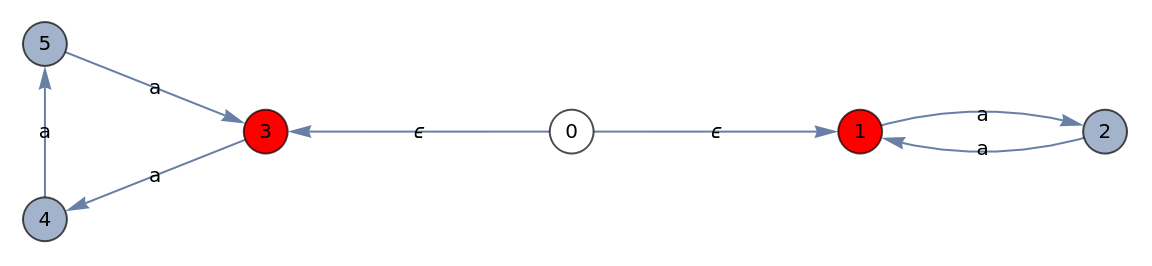
Transition Table:
In[]:=
FATable[δ,{0,1,2,3,4,5},{ϵ,"a"}]
Out[]=
Q\Σ | ϵ | a |
0 | {1,3} | - |
1 | - | {2} |
2 | - | {1} |
3 | - | {4} |
4 | - | {5} |
5 | - | {3} |
Evaluation:
In[]:=
DeltaHat[δ,{0},"aaa"]
Out[]=
{{0,1,3},{2,4},{1,5},{2,3}}
In[]:=
IsValidQ[δ,{0},{1,3},"aaa"]
Out[]=
True
Example 2
Example 2
Strings Accepted: Accepts strings that start and finish with “a”, or start and finish with “b”. Starting state 0, final states {1,3}
Definition:
In[]:=
δ=Association[{0,"a"}{1},{0,"b"}{3},{1,"a"}{1},{1,"b"}{2},{2,"b"}{2},{2,"a"}{1},{3,"b"}{3},{3,"a"}{4},{4,"b"}{3},{4,"a"}{4}];
Graph :
In[]:=
ShowGraphFA[{01,03,11,12,22,21,33,34,43,44},{0,1,2,3,4,5},{0},{1,3},{"a","b","a","b","b","a","b","a","b","a"},ImageSize->Large]
Out[]=

Transition Table:
In[]:=
FATable[δ,{0,1,2,3,4},{"a","b"}]
Out[]=
Q\Σ | a | b |
0 | {1} | {3} |
1 | {1} | {2} |
2 | {1} | {2} |
3 | {4} | {3} |
4 | {4} | {3} |
Evaluation:
Example 3
Example 3
Strings Accepted
Strings Accepted
Accepts strings that end in 1. initial state 0, final state 1
Definition
Definition
Graph
Graph
Transition Table
Transition Table
Evaluation
Evaluation
Example 4
Example 4
Strings Accepted: Accepts binary strings that are integers multiples of 4 in binary notation. Starting state 0, final state 0
Graph :
Transition Table:
Evaluation:
Example 5
Example 5
Strings Accepted:
Strings Accepted:
Contains at least one 1 and a pair number of 0 after the last 1.
Definition:
Definition:
Graph :
Graph :
Transition Table:
Transition Table:
Evaluation:
Evaluation:
Example 6
Example 6
Strings Accepted:
Strings Accepted:
Accepts decimal numbers with an optional “+“ or “-“, followed by a sequence of integers digits, a point and another sequence of integer digits. The initial state is 0 and the final state 5.
Definition:
Definition:
Graph :
Graph :
Transition Table:
Transition Table:
Evaluation:
Evaluation:
Example 7
Example 7
Strings Accepted:
Strings Accepted:
Accepts expressions that contain “ebay” or “web”. Initial state 0, final states {3,7} . The alphabet is all small English letters and space.
Definition:
Definition:
Graph :
Graph :
Transition Table:
Transition Table:
Evaluation:
Evaluation:
Example 8
Example 8
Strings Accepted:
Strings Accepted:
Accepts a sum of symbols 0 Modulo 3. “r” resets de count to 0. Star state is 0, final state is 0
Definition:
Definition:
Graph :
Graph :
Transition Table:
Transition Table:
Evaluation:
Evaluation:
Example 9
Example 9
Strings Accepted:
Strings Accepted:
Accepts strings that contain a sequence “001”. Start state 0, final state 3.
Definition:
Definition:
Graph :
Graph :
Transition Table:
Transition Table:
Evaluation:
Evaluation:
References
References
◼
Hopcroft and Ullman, Introduction to Automata Theory, Languages and Computation, Addison Wesley.
◼
Michael Sipser, Introduction to theTheory of Computation. PWS Publishing Company, 2006.