Abstract
Abstract
The amount of substance left after a radioactive decay can be calculated by solving differential equations, the solutions to which represent exponential decays over time. In this project, I develop functions that are used to generate the decay chain and calculate the amount of each element left after a given time. Most of the functions defined make use of the graph at the start, and derive sources, products, and paths from it. We can also compare the amount of different elements remaining after a certain time.
Overview of Calculations
Overview of Calculations
As opposed to other traditional methods, this program does not use the explicit forms of the Bateman equations to solve for decay products. Instead, I derive another form from the simple equation for radioactive decay. We know that for a single radioactive isotope of decay constant λ, starting with x quantity, the amount remaining after a certain time is given by the exponential decay:
N(t) = x
-λt
Now consider the amount of product. Suppose the above substance decays into another substance with branching ratio a (number between 0 and 1). As we used x above, this time the initial amount will be the amount of decayed source. Thus, the amount of this substance remaining after a certain time will be,
N
2
-t
λ
2
N
2
-λt
-t
λ
2
N
2
-λt
-t
λ
2
Here, is the decay constant of the product. We can see the pattern here: the amount of substance left after a certain time is the branching ratio times the difference between initial amount of the source and amount of source as a function of time times the decaying exponential for the substance. This can be generalized to work for any element in the chain. The initial amount x becomes a function of time, based on the decay of the source. Therefore,
λ
2
N
i
a
i
x
i-1
-t
λ
i-1
-t
λ
i
Here, the index i refers to the terms corresponding to the substance in question, and i-1 corresponds to its source. is the percentage of the source that gets converted to the product (branching ratio).
a
i
Graphing the Decay Chain
Graphing the Decay Chain
Before we get to any calculations, let us define the decay chain. This would be a Graph object containing Directed Edges from source to product. This is important to define the relationship between different elements of the chain, and is used extensively in this program.
We start a general function to create a graph object
We start a general function to create a graph object
In[]:=
dNuclides[ele_]:=Flatten[Select[ele["DaughterNuclides"],MissingQ[#]False&]];chainPlot[subs_]:=Module[{l2},l2=Flatten[NestWhileList[Flatten[dNuclides/@#]&,{subs},dNuclides/@#=!={}&]];SimpleGraph[Graph[Tooltip/@l2,DeleteMissing[Union[Flatten[Thread[##["DaughterNuclides"]]&/@l2]]]],GraphLayout"LayeredEmbedding"]]
The function dNuclides is defined above for convenience: it simply generates the list of daughter nuclides of the given element and can be mapped across a list. Right below it, chainPlot takes in the Isotope Entity to create the actual plot.
It first uses NestWhileList and Flatten to create the list of all isotopes involved in the decay. It then generates the plot by threading together the generated list (with duplicates deleted by Union) with each element's daughter nuclides. This creates the list of Directed Edges that are used with Graph to create the chain diagram.
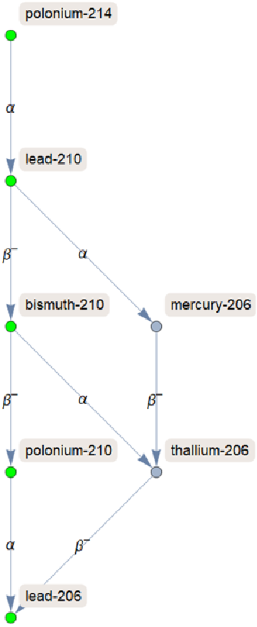
Let us test this with Polonium-214.
It first uses NestWhileList and Flatten to create the list of all isotopes involved in the decay. It then generates the plot by threading together the generated list (with duplicates deleted by Union) with each element's daughter nuclides. This creates the list of Directed Edges that are used with Graph to create the chain diagram.
Let us test this with Polonium-214.
In[]:=
g=chainPlot[Entity["Isotope","Polonium214"]];HLList[g_,source_]:=Module[{finals,branches},finals=Select[VertexList[g],Length[VertexOutComponent[g,{#}]]1&];branches=Flatten[allPaths[g,source,#]&/@finals,1];branches[[Position[branches[[All,2]],Max[branches[[All,2]]/.Missing["Unknown"]0]][[1,1]],1]]]
Another thing to note is that for visuals, I defined a function HLList that is used with VertexStyle to highlight the main decay branch in the graph. It uses a function allPaths which I have defined and put in an initialization cell in the next section, but a simple explanation is that it multiplies together the branching ratios for all possible paths between the source element and the final products, and returns the chain with the largest product of branching ratios (ie. the one with the most contribution).
Thus, the main decay branch is highlighted green in the image below.
Thus, the main decay branch is highlighted green in the image below.
In[]:=
SimpleGraph[Graph[EdgeList[g]],VertexLabels"Name",EdgeLabelsThread[(EdgeList[g])(EdgeList[g][[#]][[1]]["DecayModeSymbols"][[Position[EdgeList[g][[#]][[1]]["DaughterNuclides"],EdgeList[g][[#]][[2]]][[1,1]]]]&/@Range[Length[EdgeList[g]]])],VertexStyleThread[HLList[g,Entity["Isotope","Polonium214"]]Green],ImageSizeMedium]
Out[]=
Calculating Decay Product amounts
Calculating Decay Product amounts
Now for the functions that are actually used to calculate the amounts of each element.
In[]:=
f[{a_,b_}]:=(a["BranchingRatios"][[Position[a["DaughterNuclides"],b][[1,1]]]]);allPaths[g1_,el1_,el2_]:=Module[{ap},ap=FindPath[g1,el1,el2,Infinity,All];Thread[{ap,(If[QuantityQ[(Times@@(BlockMap[f,ap[[#]],2,1]))]True,QuantityMagnitude[(Times@@(BlockMap[f,ap[[#]],2,1]))]/100,(Times@@(BlockMap[f,ap[[#]],2,1]))]&/@Range[Length[ap]])}]]
The first part is to calculate the all the possible paths, and the percentage of products that actually follow that decay chain. The function defined uses the FindPath function on a graph, along with the start and end points to determine all possible paths between them. Then, BlockMap is used on pairs of elements of each path to determine the branching ratio of each edge, and multiply them all together.
A thing to note here is that a function is mapped across a Range[]. This runs much faster than a For[] loop, while producing the same functionality. I use this to map functions across lists in multiple places in the full program.
A thing to note here is that a function is mapped across a Range[]. This runs much faster than a For[] loop, while producing the same functionality. I use this to map functions across lists in multiple places in the full program.
In[]:=
fx[a_,{b_,c_}]:=a-a*Exp[-t*QuantityMagnitude[b["DecayConstant"]]]timeDecay[substance_,path_,amount_]:=Module[{testfunc},If[QuantityMagnitude[path[[-1]]["DecayConstant"]]0,testfunc=Fold[fx,amount,Partition[path,2,1]],testfunc=Fold[fx,amount,Partition[path,2,1]]*Exp[-QuantityMagnitude[path[[-1]]["DecayConstant"]]*t]]]
The next part takes in the initial amount and uses Fold and Partition to generate the amount of product as a function of time, according to the calculations in the previous section. The function fx calculates the amount of product from a pair, and this is applied to the pairs across the whole path.
In[]:=
totalPlot[graph_,source_,substance_,amount_]:=Module[{paths,ratios,decayFunctions},If[source=!=substance,ratios=allPaths[graph,source,substance][[All,2]];paths=allPaths[graph,source,substance][[All,1]];decayFunctions=Total[timeDecay[substance,paths[[#]],amount]&/@Range[Length[paths]]*ratios],amount*Exp[-t*QuantityMagnitude[substance["DecayConstant"]]]]]Off[General::munfl]Off[Part::pkspec1]Off[Part::partw]
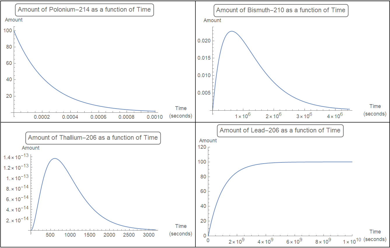
Finally, we define the function that calls the previous two functions and sums across all paths, based on the branching ratios generated by the first. I also added an If statement for the case of the source element being entered: that just contains a singe exponential decay. Now we can test this out for some components of the graph. Here's an example of using the totalPlot function to plot four of the isotopes in the chain (the domain of the plot for Polonium-214 is set to [0, 0.001] since it has an incredibly short half life of 164.1 μs):
In[]:=
p11=Plot[totalPlot[g,Entity["Isotope","Polonium214"],Entity["Isotope","Polonium214"],100],{t,0,0.001},AxesLabel{" Time\n (seconds)","Amount"},PlotLabelStyle[Framed["Amount of Polonium-214 as a function of Time",RoundingRadius4]],ImageSizeMedium];p12=Plot[totalPlot[g,Entity["Isotope","Polonium214"],Entity["Isotope","Bismuth210"],100],{t,0,10^6.65},AxesLabel{" Time\n (seconds)","Amount"},PlotLabelStyle[Framed["Amount of Bismuth-210 as a function of Time",RoundingRadius4]],ImageSizeMedium];p13=Plot[totalPlot[g,Entity["Isotope","Polonium214"],Entity["Isotope","Thallium206"],100],{t,0,10^3.5},AxesLabel{" Time\n (seconds)","Amount"},PlotLabelStyle[Framed["Amount of Thallium-206 as a function of Time",RoundingRadius4]],ImageSizeMedium];p14=Plot[totalPlot[g,Entity["Isotope","Polonium214"],Entity["Isotope","Lead206"],100],{t,0,10^10},AxesLabel{" Time\n (seconds)","Amount"},PlotLabelStyle[Framed["Amount of Lead-206 as a function of Time",RoundingRadius4]],PlotRange{{0,10^10},{0,120}},ImageSizeMedium];Grid[{{p11,p12},{p13,p14}},FrameAll]
Out[]=
Visualizing Amounts for all elements
Visualizing Amounts for all elements
While it can be used for all substances, it is recommended that you plot the combined graph only for those radioactive isotopes with relatively small decay chains (<15 unique isotopes) to avoid cluttering the plot and make the plot legend readable.
In[]:=
allFunctions=totalPlot[g,Entity["Isotope","Polonium214"],VertexList[g][[#]],100]&/@Range[Length[VertexList[g]]];Manipulate[Plot[allFunctions,{t,0,10^n},PlotLegendsVertexList[g],ExclusionsNone],{n,1,20}]
Out[]=
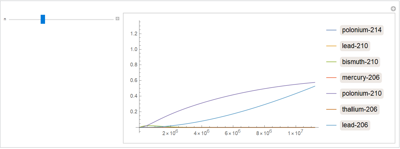
The code involved here is relatively short. The Graph object generated previously is used here again, and totalPlot is mapped across the list of vertices. The result is then plotted on a Logarithmic scale (for better visualization of all isotopes), again with the Manipulate slider.
Applications with Longer Decay Chains
Applications with Longer Decay Chains
The best part about this program is that all the functions defined here are scalable to a decay chain of any length! Here are the results for the decay chain of Radon-222.
We define the graph object as follows:
As before, we can use the totalPlot function to plot the amount of any substance. We use 4 isotopes from the decay chain as shown below:
Using this, we can find the amount of any element in the chain. Since this chain contains 17 different isotope, we won't be plotting all of them on the same plot.
Thus, the functions are able to scale appropriately to any decay chain.
Thus, the functions are able to scale appropriately to any decay chain.
Conclusion
Conclusion
Before arriving at the above result, I did the entire project using object oriented programming and class structures. Although this method provided enormous flexibility with regard to how data could be retrieved and visualized, it was incredibly slow. The initialization function was recursive, and had to assign 7 different attributes to each instance of the class. Nevertheless, it provided for quite very interesting results. The post containing the code can be found here. The method used here takes advantage of the functional nature of the Wolfram Language, and it every function defined works much faster. I ended up using the graph defined at the start as my "data structure", to retrieve all the decay chains and paths, which worked well enough.
I believe that the form of equations I used are easier to use in large scale programs than the Bateman equations. As mentioned, this program can be applied to any radioactive series, although series with over 25 different isotopes slow it down significantly. Future work can be done with optimizing the code to run faster for those cases.
Overall, the code worked out well, and I'm quite happy with the results.
I believe that the form of equations I used are easier to use in large scale programs than the Bateman equations. As mentioned, this program can be applied to any radioactive series, although series with over 25 different isotopes slow it down significantly. Future work can be done with optimizing the code to run faster for those cases.
Overall, the code worked out well, and I'm quite happy with the results.
Keywords
Keywords
◼
Radioactive
◼
Decay
◼
Nuclear
◼
Isotope