This study investigates the radiative behavior of discrete spacetime structures within the framework of the Wolfram Physics Project class of models. Different hypergraph rewriting rules are used to evolve an initially perturbed discrete spacelike hypersurface and then analyzed to determine how the spatial curvature and graph distance metric evolves, similar to how gravitational waves are studied in general relativity by perturbing the spacetime metric tensor. By analyzing the discrete analogue to gravitational waves across different Wolfram models, particularly in scenarios involving compact objects like neutron stars and black holes, this research aims to uncover potential deviations that could expand our understanding of spacetime structure at fundamental scales.
Introduction
Introduction
This work begins with a review of background material related to the subject starting with the notion of the spacetime continuum in Section 1.1, followed by a review of the relevant discoveries about radiation phenomena with a focus on gravitational waves in Section 1.2, and finally a brief overview of the Wolfram-class models and their motivation in Section 1.3.
Section 2.1 introduces potential rules with radiative behavior which are investigated on simple systems, and then the most promising rule is applied to larger and more complicated initial conditions in Section 2.2.
Section 2.1 introduces potential rules with radiative behavior which are investigated on simple systems, and then the most promising rule is applied to larger and more complicated initial conditions in Section 2.2.
1 Background
1 Background
1.1 The Continuum Paradigm
1.1 The Continuum Paradigm
Since the invention of calculus in the 1600s CE, the greatest advances in mathematical physics have been made through the analysis of particle, field, and quantum mechanics on a continuous spacetime manifold, or what might be called the spacetime continuum. Ironically, the assumption of spacetime continuity has led to a discontinuity within the current scientific paradigm. The most successful theories of modern physics are General Relativity and Quantum Field Theory (the latter is often considered a class of theories), but the two are incompatible at small scales [1]. The theories are quite successful in the appropriate settings, but there are no reasonable interpretations of black hole singularities, dark matter, dark energy, or the origin of physical constants in these models. These issues suggest that spacetime might have a discrete structure from which these unexplained features emerge. The purpose of this current work is to determine whether or not a discrete spacetime could produce observable signatures in gravitational waves distinguishable from the results obtained through analysis with the continuum assumption.
1.2 Types of Radiation in the Continuum Limit
1.2 Types of Radiation in the Continuum Limit
Electromagnetic and Weak
Electromagnetic and Weak
Radiation is a phenomenon which is most familiar from the study of electromagnetism. Maxwell’s unification of electric and magnetic forces led physicists to picture radiation as a wave in the electromagnetic field responsible for transmitting energy between electrically charged particles. Certain frequencies of these waves are perceived by us as light.
It is now well understood that light can only be detected in discrete quantities, and so it is more natural to think about light as a collection of photons (discrete objects, each of which carries a discrete amount of energy) interacting with electrically charged particles such as electrons. The theory which describes how photons interact with matter is called Quantum Electrodynamics (QED), and it is an example of a quantum field theory [2].
Stars like the sun produce energy through nuclear fusion reactions in their cores. All life on Earth depends on the persistent energy output of the sun in the form sunlight. The sun is more powerful than lightbulbs operating at 100 Watts (W).
24
10
Mathematica’s database contains the luminosity of the sun:
In[]:=
Out[]=
Nuclear fusion reactions in the sun also produce weakly interacting particles called neutrinos which can be detected in specially designed detectors on Earth. Trillions of neutrinos pass through your body every second. The Super-Kamiokande experiment uses over 10 million gallons (50 thousand tons) of ultra-pure water to detect the small fraction of neutrinos which happen to interact with matter on Earth [3]. Neutrino radiation is most important physically in supernovae and the big bang. During the first second after the big bang, the universe was hot enough that the electromagnetic and weak forces were united into a single “electro-weak” interaction. The discovery of this unification predicted by quantum field theorists and verified in particle accelerators gives physicists renewed hope that all of the forces of nature might be described by a single Grand Unified Theory.
Gravitational
Gravitational
What is much less familiar of a phenomenon than light is gravitational radiation. In the context of general relativity, the propagation of a gravitational wave can be thought of as a ripple in spacetime resulting in oscillating tidal deformations transverse to the direction of propagation. We can investigate the properties of gravitational waves by simply perturbing the flat Minkowski spacetime metric, and then solving Einstein’s field equations in vacuum.
The perturbation below is the general form for a wave propagating in the z direction and polarized along the x- and y-axes [4 p.16-14]:
The perturbation below is the general form for a wave propagating in the z direction and polarized along the x- and y-axes [4 p.16-14]:
2
dτ
2
dt
2
dx
2
dy
2
dz
(
1
)G
μν
(
2
)When this perturbation term h is explicitly solved in the case of two objects of mass and orbiting each other at a distance r in the x-y plane, then the result is purely a function of the coordinates t and z [4 p.16-19]:
M
1
M
2
h(t,z)=-rzcos2(+)-t
4
2
M
1
M
2
4
1/2
M
1
M
2
3
r
z
(
3
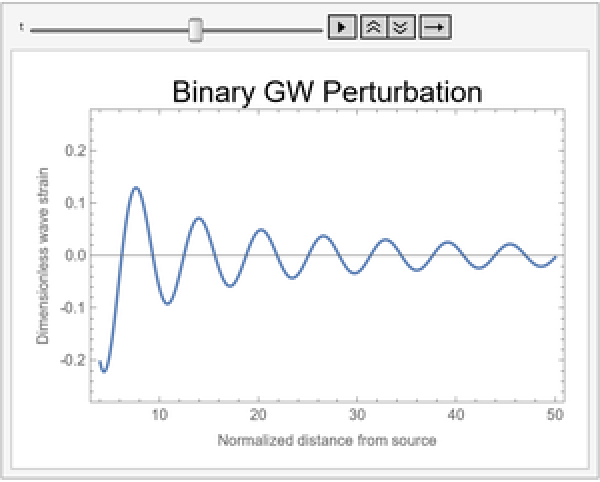
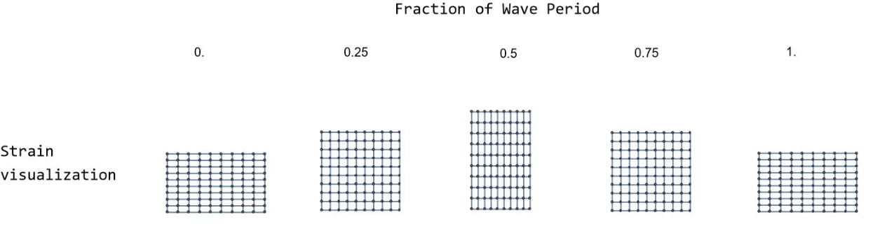
)The term h is called the wave strain, because an observer measuring distances in the x-axis will observe that they are stretched/compressed by a factor of (1 + h/2), and similarly along the y-axis they will measure compressed/stretched distances by a factor of (1 - h/2). This is the principle of how gravitational wave observatories such as LIGO operate; they use interferometry to measure differences in distances along two perpendicular arms. One important note is that no detection will be made if the gravitational wave is polarized at a 45° angle with respect to the arms, since the strain will effect both arms equally in that case. That is partly why signals from multiple observatories must be combined. Below is an animation of how the wave perturbation evolves with all constants set to one:
In[]:=
h[t_,z_]:=-Cos[z-t]/z;Animate[Plot[h[t,z],{z,4,50},PlotRange->0.28,FrameLabel{"Normalized distance from source","Dimensionless wave strain"},FrameTrue,PlotLabelStyle["Binary GW Perturbation",20,Black],ImageSizeMedium],{t,0,30},ControlPlacement->Top,AnimationRunning->False,SaveDefinitions->True]
Out[]=
Below is a diagram showing an exaggerated view of how a 2-dimensional slice of space is deformed as a gravitational wave passes through perpendicular to it:
The detection of gravitational waves is less noticeable than electromagnetic waves for at least two reasons. The first reason is that a spherical distribution of matter (such as a single star or a static black hole) can never produce gravitational radiation unless it develops some asymmetry. The second reason is that even when some asymmetric system produces these gravitational disturbances, the energy which is radiated out is often small compared to light sources and the waves do not interact strongly with matter. The fact that gravitational waves are so weakly interacting is actually also a benefit for detection purposes because it means the signal will not be distorted by intervening matter, unlike light which is frequently blocked by interstellar dust. These constraints explain why the only currently detectable gravitational radiation originates from massive compact binary systems. However, it is thought that there are other astrophysical sources of gravitational waves including pulsars, supernovae, and even background gravitational waves from the Big Bang (analogous to Cosmic Microwave Background Radiation) [5 p .246]. The next generation of detectors may be sensitive to these sources.
By considering the effective contribution of the perturbation to the stress-energy tensor, it is possible to derive a formula for the amount of gravitational energy lost per unit time in a binary system. The result is known as Einstein’s quadrupole formula. By assuming circular orbits, we can derive the formula below for calculating the power emitted in gravitational radiation by a binary system given the masses and their separation [4 p.16-18]:
L
GW
32(+)
4
M
1
M
2
2
()
M
1
M
2
5
5
5
r
(
4
)These functions return the wave strain amplitude (at a certain distance), frequency, and luminosity of gravitational radiation in a binary system given the masses and separation:
In[]:=
gravitationalWaveAmplitude[M1_,M2_,r_,z_]:=rzgravitationalWaveFrequency[M1_,M2_,r_]:=UnitConvert[(M1+M2),"Hertz"]gravitationalWaveLuminosity[M1_,M2_,r_]:=UnitConvert[,"Watts"]gravitationalWaveProperties[M1_,M2_,r_]:=<|"Amplitude at 1 ly"->gravitationalWaveAmplitude[M1,M2,r,],"Frequency"->gravitationalWaveFrequency[M1,M2,r],"Luminosity"gravitationalWaveLuminosity[M1,M2,r]|>
4M1M2
2
4
1
π
3
r
32(M1+M2)
4
2
(M1M2)
5
5
5
r
Below is a table of these properties generated for different binary systems:
In[]:=
Dataset[<|"Earth-Moon"->gravitationalWaveProperties[[],[],[]],"Sun-Jupiter"->gravitationalWaveProperties[[],[],[]],"Two stars at 1 au"->gravitationalWaveProperties[[],[],],"Two 3 neutron stars at 100 km"->gravitationalWaveProperties[3[],3[],],"Two 60 black holes at 1000 km"->gravitationalWaveProperties[60[],60[],]|>,HeaderSize20,ItemDisplayFunction{"Amplitude at 1 ly"(ScientificForm[#]&)}]
M
☉
M
☉
M
☉
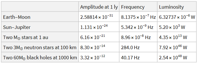
We can see that the luminosity of the gravitational radiation can range from less than twenty orders of magnitude less than the luminosity of the sun to over twenty orders of magnitude greater. The reason for the dramatic changes in the power output is that the luminosity of the gravitational waves in a binary system varies inversely with the fifth power of the separation distance. That means that if the separation is halved, then the gravitational waves will be 32 times more powerful.
Binaries radiate gravitational energy and begin to in-spiral towards their center of mass. As they get closer, they radiate more strongly and therefore approach each other even faster. The time it will take for them to collide is again just a simple function of their masses and initial separation derivable through the equations above (and a little calculus) [4 p.16-22]:
t
inspiral
5
5
4
r
initial
256(+)
4
M
1
M
2
M
1
M
2
(
5
)Since the separation of the binary decreases during the in-spiral phase, both the luminosity and frequency will increase dramatically. The frequency of the wave enters into the audible range of human hearing in the last few seconds, and gives off a distinctive “chirp”. The evolution of the frequency is best defined by a parameter called the chirp mass [6]:
M
chirp
3/5
()
M
1
M
2
1/5
(+)
M
1
M
2
(
6
) f=
3/8
5
8π
5/8
3
M
chirp
-3/8
-t
t
inspiral
(
7
)Useful functions for in-spiral characteristics, including generating audio from their frequency:
In[]:=
inspiralTime[M1_,M2_,rinit_]:=UnitConvert[,"Seconds"]chirpMass[M1_,M2_]:=UnitConvert[,"SolarMass"]frequencyEvolution[M1_,M2_,rinit_,t_]:=UnitConvert[,"Hertz"]generateInspiralAudio[M1_,M2_,rinit_,model_:"Square"]:=Module[{freq,tfinal,vib},freq[t_]:=QuantityMagnitude@frequencyEvolution[M1,M2,rinit,t];tfinal=QuantityMagnitude@inspiralTime[M1,M2,rinit]-0.001;vib=TimeSeries[Table[{t,freq[t]},{t,0,tfinal,1/200}]];AudioGenerator[{model,vib},SampleRateAutomatic]]
5
5
4
rinit
256M1M2(M1+M2)
3
3/5
(M1M2)
1/5
(M1+M2)
3/8
5
8π
5/8
(chirpMass[M1,M2])
3
-3/8
(inspiralTime[M1,M2,rinit]-Quantity[t,"Seconds"])
These audio clips based on the theoretical prediction of general relativity are how the data collected by LIGO of merger events actually “sound” (see here, for instance), and this is a remarkable achievement of modern physics. Black hole mergers happen much faster than neutron stars so the frequency of their waves are in the audible range for a much shorter time, although the square wave audio generator still makes a sound which resembles two magnets colliding and “ringing down”. It is also important to note that because LIGO uses an interferometer with freely swinging mirrors, there are significant sources of thermal and mechanical noise on the ground which limit LIGO’s sensitivity to frequencies between 10 Hz and 10,000 Hz. Now that gravitational waves have been detected the next step is to use more sensitive instruments to probe gravitational radiation even further. The LISA instrument will be a gravitational wave detector operating in space which may allow for enough precision to discover new properties of these compact binary systems. There could even be signatures which provide evidence of gravitons or the background gravitational radiation from the early universe [5 p .242].
1.3 Motivation for Discreteness
1.3 Motivation for Discreteness
It is possible that gravitational waves are composed of discrete transmitters of gravitational energy called gravitons, analogous to how electromagnetic waves are composed of photons. There has been no successful theoretical description of gravitons. In the Standard Model approach to quantization the graviton must be a massless spin-2 gauge boson, a particle whose quantum field is not renormalizable. The inability to renormalize the graviton field makes it impossible to build a quantum theory of gravity using the standard approach. One attractive solution to the issue is to let go of the notion of the spacetime continuum and instead try to imagine how discrete structures such as graphs and hypergraphs may evolve in a way which resembles gravitation. This is one of the primary motivations of the Wolfram-class models [8][9].
Ultimately the symmetries of the resulting structures in the graph will rely heavily on the symmetries of the rewriting rule used to evolve the system. The symmetries of relativistic spacetime may give us a clue as to which rewriting rules are viable candidates.
2 The Discrete Structure of a Wave
2 The Discrete Structure of a Wave
2.1 Finding the Rule(s)
2.1 Finding the Rule(s)
There are many different lattice systems whose graphs could be used as discrete structures to represent three-dimensional space. The 14 Bravais lattices are the potential candidates which have translational symmetry in Euclidean space, but there are many other examples which fill the space using different types of symmetry [10 p. 71]. All of these systems share the feature that the number of nodes within a certain number of edges from another node grows with the third power of that distance, analogous to how the volume of a sphere grows with the third power of the radius. Many of these lattice systems correspond to configurations of points in space with connections forming to their nearest neighbors. Therefore we can construct reasonable test cases by arranging points in space either randomly, regularly, or according to some perturbation and then evolving them according to different rules.
Suppose for simplicity that we just had four points in our universe, and that the only states that they could assume were simply connected graphs:
The most interesting of these universes are in the bottom row. We have the cycle graph, the diamond graph, and the complete graph on four vertices, respectively. In the cycle graph the top/bottom and left/right pairs are each a graph distance of 2 away from each other, in the diamond graph the vertical distance is now 1 while the horizontal is still 2 and in the complete graph both distances are 1. The diamond graph is therefore an attractive representation of how a gravitational wave deforms space. We can imagine a graviton as following a certain rule which transports it through a three-dimensional lattice. One significant limitation of this rule is that it seems to require a spacetime structure which is preferential to certain directions or polarizations of these waves. For instance it is not yet clear whether this rule can produce waves polarized 45 degrees with respect to the symmetry axes. However, at this level of abstraction there is still significant insight to be gained by imposing some structure on the spacetime before trying to generalize the rule.
To construct our graph rewrite rule, we look for a diamond graph where the connected corners have extraneous edges along which we can slide the center edge down, thereby transporting it down the lattice and leaving a cycle graph where it was before. This example assumes that the underlying flat structure of space is a cubic lattice:
To avoid getting stuck with larger lattices, we should make sure we have directed edges in both directions to maintain the symmetry of the setup and ensure that our model gravitons can propagate in any direction. This is equivalent to defining rules which work for any edge orientation, but takes less implementation and makes it easier to deal with asymmetry in the future:
The following evaluation shows the final evolution of the system after 50 iterations, the causal connections between updating events, and the causal invariance of the system:
To see if there is a simpler model for a wave, we could instead choose to focus just on a two-dimensional slice of the space which is perpendicular to the direction in which the wave is travelling. We could then successfully define a rule that acts on just a two-dimensional slice in a manner that recreates the effect of a wave polarized in a certain orientation:
The behavior is oscillatory by design. Below the difference between vertical and horizontal graph distance is plotted over time:
Next we can analyze the behavior of the model on a larger slice of the lattice. Simple initial conditions lead to simple oscillations, while more complex initial conditions have less regular behavior. We also introduce a function for computing the discrete analogue of the wave strain to compare with the theoretical prediction of Section 1.2. The function simply takes the difference in the graph distances plotted above but normalizes it to the average of the two distances being measured. Since the wave strain is dimensionless, this definition is consistent and should represent the true wave strain in the continuum limit.
Defining functions for plotting the evolution of 3x3 lattices and their wave strain:
Simplest initial condition:
One additional edge:
Two additional edges:
While this two-dimensional slice model is an interesting simplification of the system, it does not provide any insight into how the wave might propagate in a three-dimensional region. For that reason we will use the former rule and variations of it for the analysis of different perturbations in the following section. However, it would be interesting in the future to investigate the behavior of this two-dimensional rule and variations of it.
2.2 Initial Conditions and Simulations
2.2 Initial Conditions and Simulations
Discrete hypersurface decomposition
Discrete hypersurface decomposition
This example uses a function from the Wolfram Function Repository for generating a foliation of discrete spatial hypersurfaces given a spacetime metric tensor. The initial spatial hypersurface is then taken as the initial graph to evolve via the rule found in the previous section:
Below we select sets of nodes within the central horizontal and vertical strips to see how the perturbation evolves:
The code below uses a resource function for measuring the discrete Ricci curvature scalar at every evolution and compares the curvature along the center strip in the x and y directions:
And now we plot how the discrete analogue of the wave strain evolves as measured in the standard polarization axes:
There is definitely some oscillation but it is not exactly what we are expecting. The downside of using this discrete hypersurface decomposition function is that the z coordinate is projected down and replaced with the value of the scalar curvature. In the next examples this difficulty is avoided by explicitly starting with some three-dimensional structure in our initial graph.
Nearest neighbor with distance given by perturbed metric
Nearest neighbor with distance given by perturbed metric
Here we have a natural choice of an initial condition. We start with a integer lattice and make edges between all nodes which are within a certain distance as given by the perturbed metric:
Below we color the central core of nodes based on their scalar curvature as it is defined for Wolfram models, with blue being the smallest and red the largest:
And here are the nodes across which we will measure the horizontal and vertical graph distances to compute the wave strain:
After evolving the graph we can now animate how the wave strain evolves over time and as a function of the z direction (which was not possible in the previous example):
We see some oscillatory behavior in the wave strain as expected, but the wave strain is initially zero everywhere. This suggests a different approach in which the strain starts with a large value by design. The next example achieves this goal.
Nearest neighbor with a grid stretched by metric
Nearest neighbor with a grid stretched by metric
Another natural choice of initial condition is to take the nearest neighbor graph using the Euclidean distance but using a graph which is not uniform but is instead stretched an compressed according exactly to the wave strain. Here we have done that for a full wavelength according to the form of a gravitational wave generated by a binary system:
Again we can plot the initial graph using coloration to show what the curvature looks like:
And then we select the nodes across which we expect to measure the wave strain:
Here is an animation of how the wave strain evolves over time plotted as a function of the z direction along which we expect the wave to travel:
The animation above seems to halt halfway through after an initial relaxation phase of the wave strain. It is likely that as the ‘gravitons’ in this model travel through the lattice they get stuck at the edge and cannot travel any further. Therefore the evolution of the wave strain is limited by the boundary conditions. One idea is that we can impose conditions on the boundary in effect to let it either ‘absorb’ or ‘reflect’ the gravitons instead of just freezing them in place. Of course it would also be possible to focus on a region of space which is much larger than the wavelength of the perturbation, but the computation time needed grows significantly with the size of the initial graph.
Below is a version of the initial graph with the edges which were changed by the evolution highlighted in red. This is how the cover image was created with a color negation filter applied:
Wormhole-like structure
Wormhole-like structure
For this initial setup I was wondering what would happen if I had two clusters which were connected only by a pair of edges between them acting as a bridge or a ‘wormhole’ between the two regions of space:
And here is the graph after 20 evolutions:
The clusters seem to have been jumbled up in the final evolution. We can quantify this by plotting the evolution of the global clustering coefficient, which is the fraction of paths of length two which have a third edge forming a triangle:
The clustering coefficient is reduced to two thirds of its original value as the connections of points in space diffuse across the bridge.
There are many other experiments and analyses to be done on these kinds of models, but the results here are promising despite the limitations of computational time. A more formal mathematical formulation may yield more insightful results.
Concluding Remarks
Concluding Remarks
Ultimately it is likely that the rules discussed above are already too structured to represent anything fundamental. For example, it is hard to imagine how discrete structures similar to the ones encountered above could give rise to observed symmetries of nature. However, this approach may still be a good representation of the phenomenon of gravitational radiation which emerges from some deeper structure. A truly rigorous analysis of the model will require more advanced techniques of statistical mechanics to extract information which may actually be observable on macroscopic scales. This analysis will likely proceed similarly to the Debye model of atomic lattice vibrations or phonons [11]. The difficulty with this extension of the Debye model is the fact that the nodes in our graph must act more like a liquid than a crystalline solid in order for the edge connections to be shifted in the proposed way. This introduces nonlinear contributions to vibrations which make the analysis more difficult, but the nonlinearity is essential if the model is supposed to approximate Einstein’s field equations in the appropriate limit.
When considering the graphs to test for this project, it was necessary to impose a quasi-crystalline structure onto the spacetime from the start of the evolution in order for wave strain measurements to be well-defined. It is possible that the discrete spacetime is highly irregular on the scale of individual connections, and that it is only the macroscopic statistical behavior which has regularity. There is another reason to doubt the cubic lattice model as being fundamental. According to a definition of a graph’s dimension proposed by Oliver Knill, a cubic lattice of any size is a one-dimensional object in the sense that the set of neighbors of any node in the lattice induces a subgraph with no edges (i.e. there are no triangles) [12]. This suggests that perhaps the true structure of spacetime contains many tetrahedra or cliques of size four, since these are the simplest three-dimensional subgraphs or simplices by Knill’s definition.
The results of this model are promising but should be taken as a proof of concept rather than a complete description of discrete gravitational waves. There is much work to be done both on theoretical and experimental sides of the field to confirm or deny the validity of discretizing gravitational radiation.
Acknowledgments
Acknowledgments
I would like to thank my mentors, Gianmarco Morbelli and Jon Lederman, for their continued support and helpful insight. I also appreciate all of the administrators, speakers, and teachers at Wolfram Summer School 2024 for making this project possible and I extend my special thanks to Stephen Wolfram for suggesting this project. Finally I would like to thank Brent Corbin for introducing me to the Wolfram Language and the beauty of symbolic computation.
References
References
1
.A. Macías et al. (2008), “On the incompatibility between quantum theory and general relativity,” Physics Letters B. https://doi.org/10.1016/j.physletb.2008.03.052.
2
.R. Feynman (1988), Quantum Electrodynamics. Princeton University Press.
3
.Y. Suzuki (2019), “The Super-Kamiokande experiment,” The European Physical Journal C. http://dx.doi.org/10.1140/epjc/s10052-019-6796-2.
4
.J. Wheeler, E. Taylor, E. Bertschinger (2019), Exploring Black Holes: Introduction to General Relativity. Pearson.
5
.B. Schutz (2009), A First Course in General Relativity. Cambridge University Press.
6
.V. Tiwari et al. (2018), “Reconstruction of Chirp Mass in the Search of Compact Binaries”, Classical and Quantum Gravity. https://doi.org/10.1088%2F0264-9381%2F33%2F1%2F01LT01.
7
.Gerard ’t Hooft et al. (1974), “One loop divergencies in the theory of gravitation,” Annals of the Institut Henri Poincare. https://www.researchgate.net/publication/234365133_One-loop_divergencies_in_the_theory_of_gravitation.
8
.S. Wolfram (2020), “A Class of Models with the Potential to Represent Fundamental Physics,” Complex Systems. https://doi.org/10.25088/ComplexSystems.29.2.107.
9
.J. Gorard (2020), “Some Relativistic Properties of the Wolfram Model,” Complex Systems. https://doi.org/10.25088/ComplexSystems.29.2.599.
10
.N. Ashcroft, N. Mermin (1976), Solid State Physics. Saunders College Publishing.
11
.G. Srivastava (2019), The Physics of Phonons. Routledge.
12
.O. Knill (2011), “A Graph Theoretical Gauss-Bonnet-Chern Theorem,” ArXiv. https://doi.org/10.48550/arXiv.1111.5395.
Cite This Notebook
Cite This Notebook