We compute the number of equilibrium stages using the Hunter and Nash graphical method of a liquid liquid extraction problem. One feed of acetic acid (35 wt %) in water which flow rate = 1000 kg/hr is extracted using a solvent consisting of pure isopropyl ether which flow rate = 1475 kg/h. The exiting raffinate stream specification is 10 wt % acetic acid.
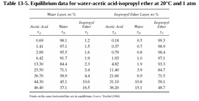
Liquid Liquid Equilibrium of ternary system Isopropyl Ether-Water-Acetic Acid (data are given in wt. frac.).Component 1 = Water Component 2 = Acetic AcidComponent 3 = Isopropyl EtherABREVIATIONS:Water = WAcetic Acid = AAIsopropyl Ether = IE
In[]:=
tbl1={{98.1,0.69},{97.1,1.41},{95.5,2.89},{91.7,6.42},{84.4,13.30},{71.1,25.50},{58.9,36.70},{45.1,44.30},{37.1,46.40}};
In[]:=
tbl2={{0.5,0.18},{0.7,0.37},{0.8,0.79},{1.0,1.93},{1.9,4.82},{3.9,11.40},{6.9,21.60},{10.8,31.10},{15.1,36.20}};
In[]:=
data1=Table[{tbl1[[i]][[1]],tbl1[[i]][[2]],100-tbl1[[i]][[1]]-tbl1[[i]][[2]]},{i,1,Length[tbl1]}]
Out[]=
{{98.1,0.69,1.21},{97.1,1.41,1.49},{95.5,2.89,1.61},{91.7,6.42,1.88},{84.4,13.3,2.3},{71.1,25.5,3.4},{58.9,36.7,4.4},{45.1,44.3,10.6},{37.1,46.4,16.5}}
In[]:=
data2=Table[{tbl2[[i]][[1]],tbl2[[i]][[2]],100-tbl2[[i]][[1]]-tbl2[[i]][[2]]},{i,1,Length[tbl2]}]
Out[]=
{{0.5,0.18,99.32},{0.7,0.37,98.93},{0.8,0.79,98.41},{1.,1.93,97.07},{1.9,4.82,93.28},{3.9,11.4,84.7},{6.9,21.6,71.5},{10.8,31.1,58.1},{15.1,36.2,48.7}}
In[]:=
Pt={{2,1}/2.,{0,Sqrt[3.]}/2};(*transformationfromrectangulartoequilateral*)
In[]:=
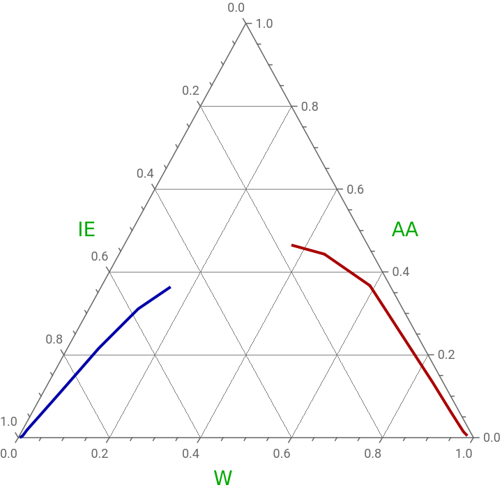
plt1=Show[TernaryListPlot[{data1,data2},JoinedTrue,PlotStyle{{Thick,Darker@Red},{Thick,Darker@Blue}},AspectRatio1,GridLinesAutomatic,Frame->True],Graphics[{Text[Style["W",14,Darker@Green],Pt.{0.5,-0.1}],Text[Style["IE",14,Darker@Green],Pt.{-0.1,0.5}],Text[Style["AA",14,Darker@Green],Pt.{0.6,0.5}]}]]
Out[]=
In[]:=
tbl1={{98.1,0.69},{97.1,1.41},{95.5,2.89},{91.7,6.42},{84.4,13.30},{71.1,25.50},{58.9,36.70},{45.1,44.30},{37.1,46.40}}/100
Out[]=
{{0.981,0.0069},{0.971,0.0141},{0.955,0.0289},{0.917,0.0642},{0.844,0.133},{0.711,0.255},{0.589,0.367},{0.451,0.443},{0.371,0.464}}
In[]:=
tbl2={{0.5,0.18},{0.7,0.37},{0.8,0.79},{1.0,1.93},{1.9,4.82},{3.9,11.40},{6.9,21.60},{10.8,31.10},{15.1,36.20}}/100
Out[]=
{{0.005,0.0018},{0.007,0.0037},{0.008,0.0079},{0.01,0.0193},{0.019,0.0482},{0.039,0.114},{0.069,0.216},{0.108,0.311},{0.151,0.362}}
In[]:=
rafnt=Evaluate[Interpolation[tbl1,InterpolationOrder1]]
Out[]=
InterpolatingFunction


In[]:=
rafnt[0.90]
Out[]=
0.0802219
In[]:=
Extrc=Evaluate[Interpolation[tbl2,InterpolationOrder1]]
Out[]=
InterpolatingFunction

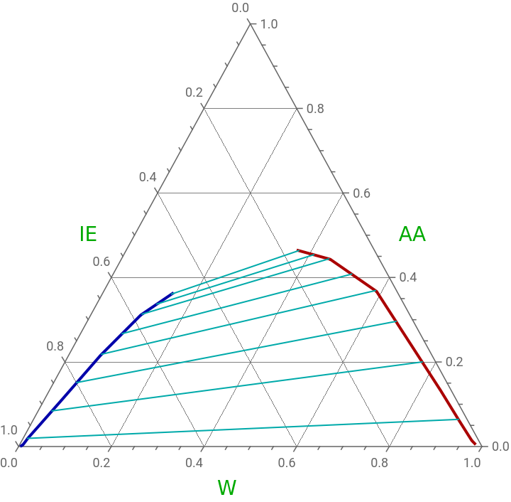
Using interpolation to get tie lines
In[]:=
tbl3={{0.5,98.1},{0.7,97.1},{0.8,95.5},{1.0,91.7},{1.9,84.4},{3.9,71.1},{6.9,58.9},{10.8,45.1},{15.1,37.1}}/100;
In[]:=
tie1=Interpolation[tbl3,InterpolationOrder1]
Out[]=
InterpolatingFunction

In[]:=
tbl4={{98.1,0.5},{97.1,0.7},{95.5,0.8},{91.7,1.0},{84.4,1.9},{71.1,3.9},{58.9,6.9},{45.1,10.8},{37.1,15.1}}/100;
In[]:=
tie2=Interpolation[tbl4,InterpolationOrder1]
Out[]=
InterpolatingFunction

In[]:=
tbl5=Table[Line[{Pt.{i,Extrc[i]},Pt.{tie1[i],rafnt[tie1[i]]}}],{i,1/100,15/100,2/100}]
Out[]=
{Line[{{0.01965,0.0167143},{0.9491,0.0555988}}],Line[{{0.072195,0.0730839},{0.8709,0.173292}}],Line[{{0.1257,0.131116},{0.8143,0.256401}}],Line[{{0.179218,0.189171},{0.769936,0.319519}}],Line[{{0.223577,0.231362},{0.718654,0.353272}}],Line[{{0.266686,0.271388},{0.669267,0.384495}}],Line[{{0.298547,0.291931},{0.636942,0.392954}}],Line[{{0.330407,0.312474},{0.604616,0.401413}}]}
In[]:=
Show[plt1,Graphics[{Darker@Cyan,tbl5}]]
Out[]=
Feed and Solvent
In[]:=
F=1000.;S=1475.;xF[1]=0.65;xF[2]=0.35;xF[3]=0;xS[1]=0;xS[2]=0;xS[3]=1.00;
Mixing Point
In[]:=
sol1=Solve[{MF+S,MxM[1]FxF[1]+SxS[1],MxM[2]FxF[2]+SxS[2],MxM[3]FxF[3]+SxS[3]},{M,xM[1],xM[2],xM[3]}]

Out[]=
{{M2475.,xM[1]0.262626,xM[2]0.141414,xM[3]0.59596}}
In[]:=
xM[1]=sol1[[1,2,2]]
Out[]=
0.262626
In[]:=
xM[2]=sol1[[1,3,2]]
Out[]=
0.141414
In[]:=
xM[3]=sol1[[1,4,2]]
Out[]=
0.59596
In[]:=
M=sol1[[1,1,2]]
Out[]=
2475.
Raffinate Product is such that acetic acid wt % is 10
In[]:=
xR[2]=10/100.
Out[]=
0.1
In[]:=
xR[1]=FindRoot[rafnt[x]xR[2],{x,0.80}][[1,2]]
Out[]=
0.879015
In[]:=
xR[3]=1-xR[1]-xR[2]
Out[]=
0.0209855
Extract Product
In[]:=
sys={R+EPM,xR[1]R+xE[1]EPMxM[1],xR[2]R+xE[2]EPMxM[2],xR[3]R+xE[3]EPMxM[3],Extrc[xE[1]]xE[2]}
Out[]=
EP+R2475.,0.879015R+EPxE[1]650.,0.1R+EPxE[2]350.,0.0209855R+EPxE[3]1475.,InterpolatingFunction[xE[1]]xE[2]

In[]:=
sol2=Quiet@Quiet@FindRoot[sys,{EP,1800},{R,150},{xE[1],5/100},{xE[2],15/100},{xE[3],80/100}]
Out[]=
{EP1842.97,R632.033,xE[1]0.0512402,xE[2]0.155617,xE[3]0.793143}
In[]:=
EP=sol2[[1,2]]
Operating Point
Plotting Feed, Solvent, Extract, Raffinate and Operating Point
Stepping off Stages
Plotting the Hunter and Nash Diagram. A little less than 6 stages (5.35 equilibrium stages) are needed to achieve the raffinate product requirement of 10 wt % acetic acid composition. Tie lines are shown in dashed green. Operating lines are plotted in magenta. The difference point is indicated in orange.
Checking our results
References
References
◼
[1] H. Binous, Equilibrium Staged Separations using Matlab® and Mathematica®, Chemical Engineering Education, 42(2), pp. 69-73, 2008.
◼
[2] H Binous, Liquid-liquid equilibrium and extraction using Mathematica, Computers in Education Journal, 16(1), pp. 78-81, 2006.
◼
[3] P.C. Wankat, Equilibrium Staged Separations, Prentice Hall, Englewood Cliffs, N.J. (1988). (example 18-2, pp. 595).
◼
[4] T. G. Hunter and A. W. Nash, J. Soc. Chem.Ind., (53) 95T-102T, 1934
CITE THIS NOTEBOOK
CITE THIS NOTEBOOK
Hunter and Nash Graphical Equilibrium Stage Method using Equilateral Diagrams
by Housam Binous and Ahmed Bellagi
Wolfram Community, STAFF PICKS, February 5, 2024
https://community.wolfram.com/groups/-/m/t/3116346
by Housam Binous and Ahmed Bellagi
Wolfram Community, STAFF PICKS, February 5, 2024
https://community.wolfram.com/groups/-/m/t/3116346