How Receiver Operating Characteristic Curves Work
How Receiver Operating Characteristic Curves Work


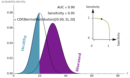
Visually the ROC curve, shown in the top-right corner, is the shaded area under the right curve versus the shaded area under the left curve as the threshold parameter varies. A more detailed explanation now follows.
Let be a possible medical diagnostic for disease. For example, , could be eye pressure and the disease could be glaucoma. We suppose that the distribution of in healthy people is and in the diseased population it is , where . These curves are shown on the left. The receiver operating characteristic (ROC) curve can be used to visualize and quantify how useful is in the detection of this disease. We suppose that people are diagnosed healthy or diseased according as or . In the above diagram, we show the case where and . The ROC curve plots sensitivity versus specificity, where
X
X
X
N(20,5)
N(μ,6)
μ>20
X
X<
X≥
μ=30
=20
sensitivity=Pr{X≥|diseased}=purpleareainplot
specificity=Pr{X<|healthy}=blueareainplot
Keeping fixed, as we vary the threshold parameter, , we trace out the ROC curve, shown in the upper-right corner. For any fixed value of , the point shown on the ROC curve corresponds to the two shaded areas.
μ
The usefulness of the test depends on . The larger is, the larger the difference between the normal and diseased populations and the easier it is to detect disease. So the diagnostic test improves if increases. The or area under the ROC curve quantifies the usefulness of the test, . Increasing increases the . For large enough , . In our Demonstration, when . In this case, the test is useless and is equivalent to simply random guessing. Obviously, when , the test, , is worse than useless!
μ
μ
μ
AUC
0<AUC<1
μ
AUC
μ
AUC≐1
AUC=0.5
μ=20
μ<20
X≥
Sometimes the ROC curve is defined as the plot of FPR versus TPR, where FPR, the false positive rate, is defined as and TPR is the true positive rate, . Click the FPR checkbox to select this type of plot. In this plot, is the area to the right of for the healthy population and is shown as the colored area under the left curve. When this area overlaps with the curve of the diseased population on the right, the blended color is shown. Similarly TPR is the area to the right of in the diseased population and is shown as the colored area under the right curve; once again the overlapping area is shown as the blended color.
FPR=1-specificity
TPR=sensitivity
FPR
Details
Details
Denote the cumulative distribution functions of in the healthy and diseased populations by (x) and (X). Then the tail functions are respectively (x)=1-(x), . It may be shown that , and
X
F
h
F
d
T
i
F
i
i=h,d
ROC(t)=(t)
T
d
-1
T
h
t∈(0,1)
AUC=ROC(t)dt
1
∫
0
An explicit closed-form formula for AUC in the case of binormal populations is given in[1], p. 34.
The AUC can be interpreted as the probability that a randomly chosen member from the diseased population will have a higher than a randomly chosen member from the healthy population.
X
An interesting example of the use of ROC curves to compare classifiers is given in[2], figure 9.6, p. 316. See also the Demonstration "Uncertainty of Measurement and Diagnostic Accuracy Measures" for an illustration of the use of ROC to compare two diagnostic tests. In practice, ROC curves are often used to compare a number of diagnostic tests or classifiers.
The glaucoma example discussed in this Demonstration is presented in[4] and there are many similar examples in the references below. Two in-depth treatments of ROC curves are provided in[1] and[3].
[1] W. J. Krzanowski and D. J. Hand, ROC Curves for Continuous Data, CRC/Chapman & Hall, 2009.
[2] T. Hastie, R. Tibshirani, and J. Friedman, The Elements of Statistical Learning: Data Mining, Inference, and Prediction, 2nd ed., New York: Springer, 2009.
[3] M.S. Pepe, The Statistical Evaluation of Medical Tests for Classification and Prediction, New York: Oxford, 2003.
[4] J. A. Swets, R. M. Dawes, and J. Monahan, "Better Decisions through Science," Scientific American, 283, 2000 pp. 82–87.
External Links
External Links
Permanent Citation
Permanent Citation
Ian McLeod
"How Receiver Operating Characteristic Curves Work"
http://demonstrations.wolfram.com/HowReceiverOperatingCharacteristicCurvesWork/
Wolfram Demonstrations Project
Published: March 7, 2011