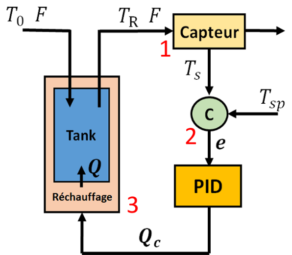
This problem was previously proposed in Ref. [1]. We would like to heat water with a heater.
1- For disturbance rejection, outlet temperature must be equal to TRset=80°C while Inlet water temperature jumps from 20°C to 30°C at t=100.
2- For setpoint change, outlet temperature must be equal to TRset=90°C starting from t=100 while Inlet water temperature is kept equal to 20°C .
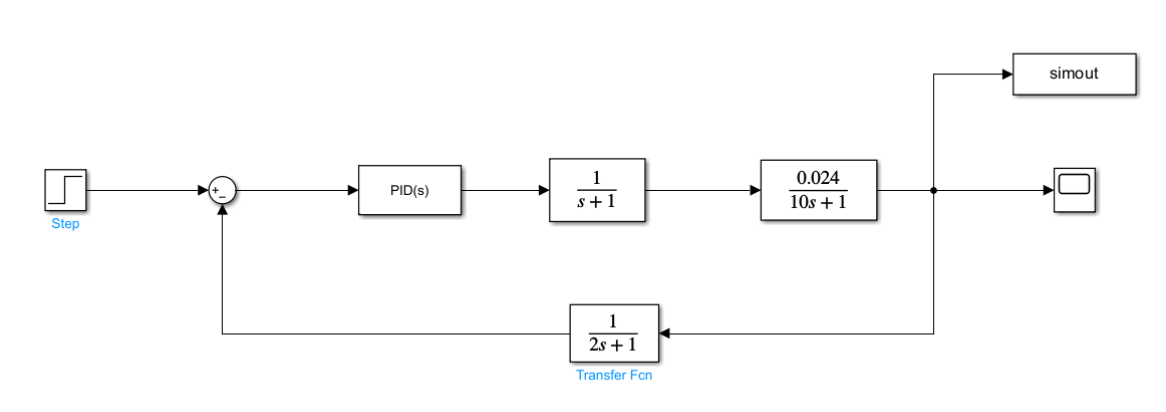
Water flow is equal to F=10 m3/hr. Tank volume is equal to V=100 m3. Water density and heat capacity are rho=1 Kg/m3 and cp=4.19 KJ/(Kg °C). The heater and the temperature measurement device have a first order delay with time constants equal to respectively TauQ=1 and TauSens=2. Nominal value of Qc (the manipulated variable) is equal to 2508 KJ/hr. The solution using Mathematica is based on either transfer functions and block diagrams or NDSolve are given in the present notebook. Finally, we successfully compare our Mathematica calculations with their counterparts obtained using Simulink.
Response to a Setpoint Change based on transfer functions and block diagram
In[]:=
Gp=TAU/(rhocpV)/(TAUs+1)
Out[]=
0.0239234
1+10s
In[]:=
TAU=10;cp=4.18;V=100;rho=1;
In[]:=
Gp
Out[]=
0.0239234
1+10s
In[]:=
Gc=KP+TAUI/s
Out[]=
300+
20.
s
In[]:=
KP=300;TAUI=20.;
In[]:=
Gc
Out[]=
300+
20.
s
In[]:=
Gs=1/(TAUSs+1)
Out[]=
1
1+2.s
In[]:=
TAUS=2.;
In[]:=
Gs
Out[]=
1
1+2.s
In[]:=
Ga=1/(TAUQs+1)
Out[]=
1
1+s
In[]:=
TAUQ=1;
In[]:=
Ga
Out[]=
1
1+s
In[]:=
G=GaGcGp/(1+GpGcGaGs)//Expand//FullSimplify
Out[]=
0.0239234+(0.406699+0.717703s)s
0.0239234+s(0.408852+s(0.65+s(1.6+1.s)))
In[]:=
Roots[0.0398724+s(0.408852+s(0.65+s(1.6+1.s)))==0,s](*allrootsofthesystem'scharacterisiticequationhavenegativerealpart-wegetastableresponse*)
Out[]=
s-1.32519||s-0.112453||s-0.0811807-0.510853||s-0.0811807+0.510853
In[]:=
LaplaceTransform[10UnitStep[t-100],t,s]
Out[]=
10
-100s
s
In[]:=
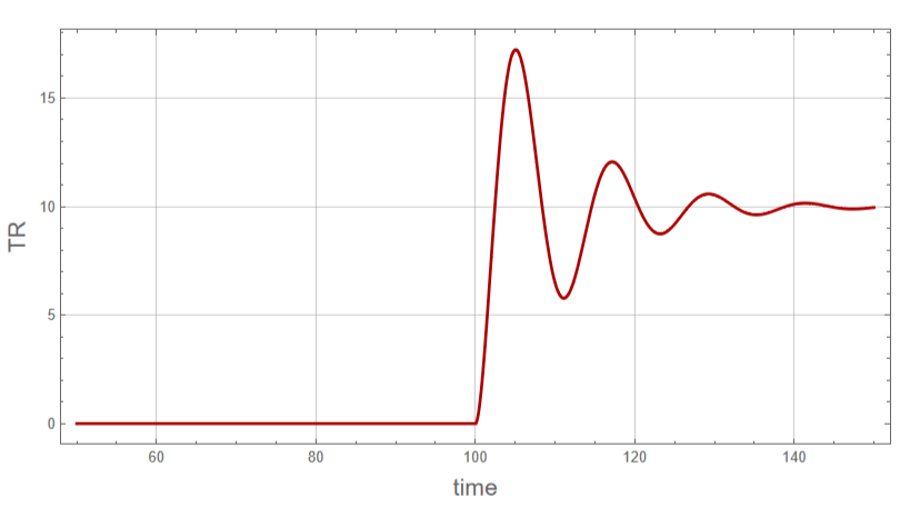
f=InverseLaplaceTransform[G10/sExp[-100s],s,t]
Out[]=
10(0.406699(-0.441909+2.90505+((-1.23157-0.628818)-(1.23157-0.628818)))HeavisideTheta[-100+t]+0.717703(0.588775-0.186064+((-0.201356+0.703941)-(0.201356+0.703941)))HeavisideTheta[-100+t]+0.0239234(41.8+0.331678-45.357+((1.61268-2.05426)+(1.61268+2.05426)))HeavisideTheta[-100+t])
-1.33234(-100+t)
-0.0640485(-100+t)
(-0.101804-0.519601)(-100+t)
(0.+1.0392)(-100+t)
-1.33234(-100+t)
-0.0640485(-100+t)
(-0.101804-0.519601)(-100+t)
(0.+1.0392)(-100+t)
-1.33234(-100+t)
-0.0640485(-100+t)
(-0.101804-0.519601)(-100+t)
(0.+1.0392)(-100+t)
In[]:=
B1=Plot[f,{t,50,150},Frame->True,GridLines->Automatic,PlotStyle->{Thick,Darker@Red},FrameLabel->{Style["time",16],Style["TR",16]},ImageSize->600{1,1},AspectRatio->0.5]
Simulink data
DataSIMULINK=;
In[]:=
A1=ListPlot[DataSIMULINK,PlotStyle->Black];
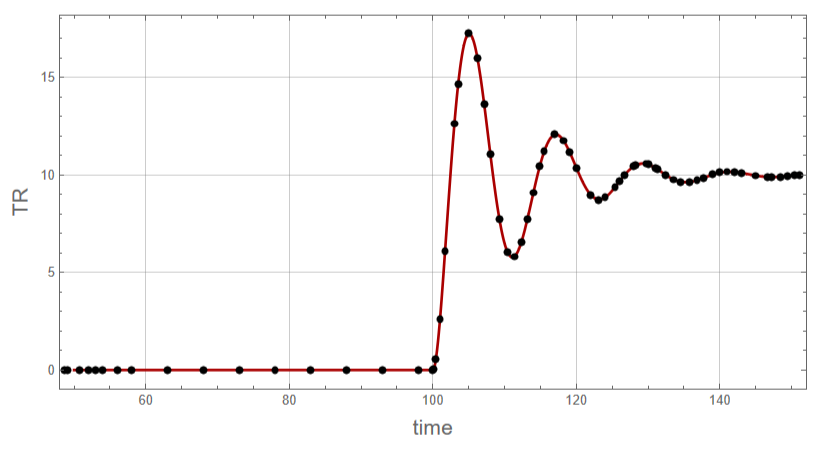
Simulink data (black dots) compared to our Mathematica result (red curve)
In[]:=
Show[B1,A1,FrameLabel->{Style["time",16],Style["TR",16]},ImageSize->600{1,1},AspectRatio->0.5]
Disturbance Rejection based on transfer functions and block diagram
In[]:=
Gd=1/(TAUs+1)
Out[]=
1
1+10s
In[]:=
G=Gd/(1+GpGcGaGs)//Expand//FullSimplify
Out[]=
0.1s(1.+s)(0.5+1.s)
0.0239234+s(0.408852+s(0.65+s(1.6+1.s)))
In[]:=
Roots[0.0398724+s(0.408852+s(0.65+s(1.6+1.s)))==0,s](*allrootsofthesystem'scharacterisiticequationhavenegativerealpart-wegetastableresponse*)
Out[]=
s-1.32519||s-0.112453||s-0.0811807-0.510853||s-0.0811807+0.510853
In[]:=
LaplaceTransform[10UnitStep[t-100],t,s]
Out[]=
10
-100s
s
In[]:=
f=InverseLaplaceTransform[G10/sExp[-100s],s,t]
Out[]=
1.(0.5(-0.441909+2.90505+((-1.23157-0.628818)-(1.23157-0.628818)))HeavisideTheta[-100+t]+1.5(0.588775-0.186064+((-0.201356+0.703941)-(0.201356+0.703941)))HeavisideTheta[-100+t]+1.(-0.784451+0.0119171+((0.386267+0.0329605)+(0.386267-0.0329605)))HeavisideTheta[-100+t])
-1.33234(-100+t)
-0.0640485(-100+t)
(-0.101804-0.519601)(-100+t)
(0.+1.0392)(-100+t)
-1.33234(-100+t)
-0.0640485(-100+t)
(-0.101804-0.519601)(-100+t)
(0.+1.0392)(-100+t)
-1.33234(-100+t)
-0.0640485(-100+t)
(-0.101804-0.519601)(-100+t)
(0.+1.0392)(-100+t)
Simulink data
Simulink data (black dots) compared to our Mathematica result (red curve)
Response to a Setpoint Change based on NDSolve
In[]:=
QC[t_]=Max[0,Q0+KP (TRset-Tsens[t])+TAUI Int[t]]
In[]:=
sol2=NDSolve[{V rho cp D[TR[t],{t,1}] F rho cp (T0-TR[t])+Q[t],
D[Q[t],{t,1}] (QC[t]-Q[t])/TauQ,
D[Tsens[t],{t,1}] (TR[t]-Tsens[t])/TauSens,
D[Int[t],{t,1}] TRset-Tsens[t],TR[0] 80,
Tsens[0] 80,Int[0] 0,Q[0] 2508},{Int[t],Q[t],
Tsens[t],TR[t]},{t,0,200}]
D[Q[t],{t,1}] (QC[t]-Q[t])/TauQ,
D[Tsens[t],{t,1}] (TR[t]-Tsens[t])/TauSens,
D[Int[t],{t,1}] TRset-Tsens[t],TR[0] 80,
Tsens[0] 80,Int[0] 0,Q[0] 2508},{Int[t],Q[t],
Tsens[t],TR[t]},{t,0,200}]
Tank temperature presents oscillatory behavior. Thus, we need to use a PID controller.
In[]:=
D1=Plot[Evaluate[TR[t]-80]/.sol2,{t,50,200},PlotStyle{Darker@Blue,Thick},PlotRangeAll,AspectRatio->1,
GridLines-> Automatic,Frame->True,FrameLabel->{Style["time",14],Style["TR",14]},ImageSize->400{1,1}]
GridLines-> Automatic,Frame->True,FrameLabel->{Style["time",14],Style["TR",14]},ImageSize->400{1,1}]
Simulink data (black dots) compared to our Mathematica result (red curve)
Disturbance Rejection based on NDSolve
In[]:=
QC[t_]=Max[0,Q0+KP (TRset-Tsens[t])+TAUI Int[t]]
In[]:=
sol2=NDSolve[{V rho cp D[TR[t],{t,1}] F rho cp (T0-TR[t])+Q[t],
D[Q[t],{t,1}] (QC[t]-Q[t])/TauQ,
D[Tsens[t],{t,1}] (TR[t]-Tsens[t])/TauSens,
D[Int[t],{t,1}] TRset-Tsens[t],TR[0] 80,
Tsens[0] 80,Int[0] 0,Q[0] 2508},{Int[t],Q[t],
Tsens[t],TR[t]},{t,0,200}]
D[Q[t],{t,1}] (QC[t]-Q[t])/TauQ,
D[Tsens[t],{t,1}] (TR[t]-Tsens[t])/TauSens,
D[Int[t],{t,1}] TRset-Tsens[t],TR[0] 80,
Tsens[0] 80,Int[0] 0,Q[0] 2508},{Int[t],Q[t],
Tsens[t],TR[t]},{t,0,200}]
Tank temperature presents oscillatory behavior. Thus, we need to use a PID controller.
In[]:=
D2=Plot[Evaluate[TR[t]-80]/.sol2,{t,50,200},PlotStyle{Darker@Blue,Thick},PlotRangeAll,AspectRatio->1,
GridLines-> Automatic,Frame->True,FrameLabel->{Style["time",14],Style["TR",14]},ImageSize->400{1,1}]
GridLines-> Automatic,Frame->True,FrameLabel->{Style["time",14],Style["TR",14]},ImageSize->400{1,1}]
Simulink data (black dots) compared to our Mathematica result (red curve)
References
References
[1] John Ingham, Irving J. Dunn, Elmar Heinzle, Jiri E. Prenosil, Jonathan B. Snape, Chemical Engineering Dynamics: An Introduction to Modelling and Computer Simulation, 3rd ed., Berlin: Wiley-VCH, 2007, pp. 420-424.
CITE THIS NOTEBOOK
CITE THIS NOTEBOOK
PI control of a heater : A comparison with Simulink results
by Housam Binous & Ahmed Bellagi
Wolfram Community, STAFF PICKS, December 9, 2024
https://community.wolfram.com/groups/-/m/t/3335540
by Housam Binous & Ahmed Bellagi
Wolfram Community, STAFF PICKS, December 9, 2024
https://community.wolfram.com/groups/-/m/t/3335540