Recent Claims by Google and Caltech/Oratomic 2026
Recent Claims by Google and Caltech/Oratomic 2026
The Wolfram Quantum Framework can simulate Shor’s full attack on elliptic curve cryptography – from oracle construction through phase estimation to key recovery. This notebook builds every step on a toy curve over GF(23), then estimates what Google’s March 2026 result means at real 256-bit scale. It also incorporates resource estimates from the Oratomic/Caltech paper which showed these same circuits can run on as few as ~10,000 neutral-atom qubits using high-rate qLDPC (quantum Low-Density Parity Check) codes, targeting the P-256 curve.
Google Quantum AI showed that the 256-bit Elliptic Curve Discrete Logarithm Problem (ECDLP) on secp256k1 can be compiled into circuits requiring ≤1,200 logical qubits and 90 million Toffoli gates, or ≤1,450 logical qubits and 70 million Toffoli gates – executable on fewer than half a million physical qubits. This is a ~20× reduction over prior estimates. The whitepaper validates these numbers via a zero-knowledge proof without disclosing the circuits.
Whitepaper: https://quantumai.google/static/site-assets/downloads/cryptocurrency-whitepaper.pdf
Blog post: https://research.google/blog/safeguarding-cryptocurrency-by-disclosing-quantum-vulnerabilities-responsibly/
Whitepaper: https://quantumai.google/static/site-assets/downloads/cryptocurrency-whitepaper.pdf
Blog post: https://research.google/blog/safeguarding-cryptocurrency-by-disclosing-quantum-vulnerabilities-responsibly/
Independently, Cain et al. at Oratomic/Caltech (arXiv:2603.28627) showed that these same ECDLP circuits can be compiled onto a neutral-atom architecture using high-rate quantum LDPC codes with ≈30% encoding rates. The paper reports a one-to-two order-of-magnitude reduction in physical qubit count compared to surface-code architectures — landing at as few as 9,739 qubits (the abstract’s ‘as few as 10,000 qubits’ headline) — at the cost of runtime: days instead of minutes.
What follows is a computation-first exploration: we define elliptic curve arithmetic as native Wolfram Language objects, build the quantum oracle using QuantumCircuitOperator and PhaseEstimation, recover a secret key, and then use the whitepaper’s data to estimate resources at scale. Every claim is backed by a WL code. You can find glossary of terms used or mentioned in this notebook at the end.
Shor’s Algorithm in One Example
Shor’s Algorithm in One Example
You can find an in-depth discussion of Shor’s factorization algorithm in my quantum computing book. In brief, Shor’s algorithm factors large integers by reducing the problem to period-finding, which a quantum computer solves exponentially faster than any known classical method. The algorithm has these steps:
◼
1. Pick a random integer a coprime to .
◼
2. Find the order : the smallest positive integer such that ≡1(mod). This is the hard step. Classically it is as hard as factoring. Quantumly it takes polynomial time.
a
◼
3. If r is even and ≢-1(mod), compute and . These are nontrivial factors of .
/2
a
gcd(-1, )
/2
a
gcd(+1, )
/2
a
◼
4. The quantum part finds : build a modular-multiplication unitary that maps , run phase estimation to sample eigenphases , recover from continued fractions.
|y〉→|y(mod)〉
k/
We demonstrate every step on with .
=15
=13
The Classical Reduction
The Classical Reduction
Verify that 13 and 15 are coprime, then find the multiplicative order:
In[]:=
=15;=13;{CoprimeQ[,],MultiplicativeOrder[,]}
Out[]=
{True,4}
It means is coprime to 15, and the order is . Since is even, compute the factors:
=13
=4
In[]:=
With[{r=4},{GCD[,PowerMod[,r/2,]-1],GCD[,PowerMod[,r/2,]+1]}]
Out[]=
{3,5}
This gives . The entire algorithm reduced to finding . That is what the quantum part does.
{3,5}
=4
The Quantum Part: Phase Estimation
The Quantum Part: Phase Estimation
We need a unitary that maps for , and acts as identity on states (padding to fill out the Hilbert space). This is the standard trick that makes the operator unitary:
|y〉→|y(mod)〉
y<
y≥
In[]:=
ClearAll[a];a[_,_]:=Module[{m=Ceiling[Log2[]]},SparseArray[{i_,j_}:>If[j-1<,KroneckerDelta[i-1,Mod[(j-1),]],KroneckerDelta[i-1,j-1]],{,}]]
m
2
m
2
For above values of and , verify is unitary:
a
In[]:=
a[,]//UnitaryMatrixQ
Out[]=
True
Verify |y〉=|y(mod)〉 with .
U
y∈{0,…,}
In[]:=
m=Ceiling[Log2[]]
Out[]=
4
Apply a to every basis state y ∈ {0, …, -1} and confirm the action matches y → y (mod ):
In[]:=
Table[a[,].UnitVector[,y+1]==UnitVector[,Mod[y,]+1],{y,0,-1}]//Apply[And]
m
2
m
2
Out[]=
True
Install quantum framework:
In[]:=
PacletInstall["https://www.wolfr.am/DevWQCF",ForceVersionInstall->True]<<Wolfram`QuantumFramework`
Out[]=
PacletObject

Consider the following phase estimation circuit for the unitary operator that implements multiplication by modulo (in this case 13 modulo 15):
In[]:=
qcShor=QuantumCircuitOperator[{"PhaseEstimation",QuantumOperator[a[,]],2m}][[m;;]];qcShor["Diagram",ImageSize->800]
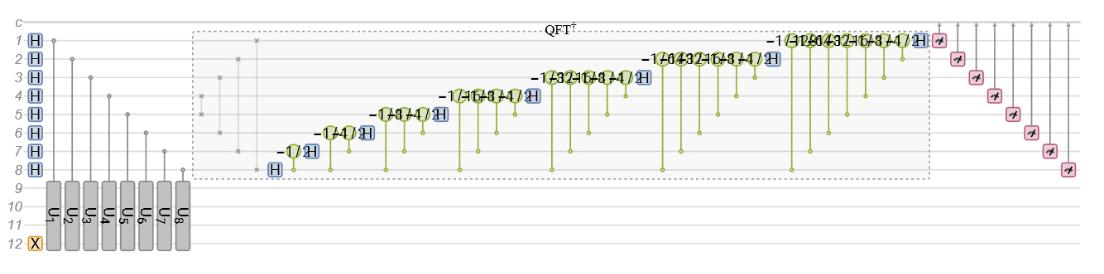
The circuit has 8 control qubits (top wires) and 4 work qubits (bottom). Each control qubit applies a controlled power of the modular multiplication unitary. The inverse QFT at the end converts accumulated phase into a measurable bitstring.
Note that 4 work qubits are prepared in the state because starting the work register in is secretly a uniform superposition over all eigenstates. Phase estimation then samples uniformly for ; exactly what the continued-fractions step needs. This is why you can break factoring without ever knowing in advance. Let’s verify that.
|0001〉
|0001〉
k/
k∈{0,…,−1}
Show that the state corresponds to integer 1:
|0001〉
In[]:=
QuantumState[QuantumState["0001"],16]//TraditionalForm
Out[]//TraditionalForm=
|1〉
𝒰ₐ is a permutation of the 16 basis states, it just shuffles them. Under repeated application it breaks the 16-dim space into disjoint cycles (orbits). The orbit containing integer 1 is {1, 13, 4, 7}: these are the only states that 𝒰ₐ can ever connect to the input . The rest of the Hilbert space is dynamically disconnected from as far as this oracle is concerned.
|y〉
|0001〉
|0001〉
Find the order containing integer 1
In[]:=
orbit=NestList[Mod[13#,15]&,1,3]
Out[]=
{1,13,4,7}
Confirm that 𝒰ₐ restricted to the orbit is a cyclic-shift operator (1 → 13 → 4 → 7 → 1):
In[]:=
a[13,15].UnitVector[16,#1+1]==UnitVector[16,#2+1]&@@@Partition[Append[orbit,orbit[[1]]],2,1]
Out[]=
{True,True,True,True}
Note is the quantity Shor’s algorithm is trying to find. By definition, r is the smallest integer with a^r ≡ 1 (mod N); equivalently, the length of the cycle that returns 1 to itself. Classically, computing r is as hard as factoring. Quantumly, phase estimation pulls it out in polynomial time. Notice that this single line “finds r” — but only because at the toy scale we can already enumerate the orbit classically. The quantum part lets us do the same thing without ever computing the orbit.
In[]:=
r=Length[orbit]
Out[]=
4
Construct the eigenvectors on the orbit as :
|〉=(mod)
k
1
r
k-1
∑
j=0
-2πjk/
j
In[]:=
uk[k_]:=(1/Sqrt[r])Sum[Exp[-2PiIjk/r]UnitVector[16,orbit[[j+1]]+1],{j,0,r-1}]
Direct verification that is an eigenvector of 𝒰ₐ with eigenvalue :
|〉
k
2πk/r
In[]:=
Table[a[13,15].uk[k]==Exp[2PiIk/r]uk[k]//Chop,{k,0,3}]
Out[]=
{True,True,True,True}
Verify Shor/Kitaev identity :
|1〉=|〉
1
r
r-1
∑
k=0
k
In[]:=
(1/Sqrt[r])Sum[uk[k],{k,0,r-1}]==QuantumState["0001"]["StateVector"]//Normal//Chop
Out[]=
True
Evaluate the circuit and get measurement outcomes:
In[]:=
meas=N[qcShor][]
Out[]=
QuantumMeasurement

Show non-zero outcomes:
In[]:=
Chop[meas]["Probability"]
Out[]=
|00000000〉0.25,|01000000〉0.25,|10000000〉0.25,|11000000〉0.25
For now, take for granted the curious fact about the distribution of sampled eigenvalues and the distribution for , where . Consider all possible outcomes that can be obtained by the previous circuit:
ϕ=
k
r
k∈{0,…,r-1}
In[]:=
Keys@meas["Probability"]
Out[]=
{|00000000〉,|01000000〉,|10000000〉,|11000000〉}
Next, convert these to fractions which uniformly estimate :
ϕ=
k
r
In[]:=
ϕs=Map&,Keys@meas["Probability"]
FromDigits[#["Name"],2]
Length[#["Name"]]
2
Out[]=
0,,,
1
4
1
2
3
4
Finally, the least common multiple of the denominators can be used to tell you :
r
In[]:=
LCM@@Denominator[ϕs]
Out[]=
4
The Pattern That Carries Over to ECDLP
The Pattern That Carries Over to ECDLP
The structure of Shor’s algorithm is: encode a hard problem as a group action, build a unitary implementing that action, use phase estimation to extract the period, then classical post-processing recovers the answer. For factoring, the group is the multiplicative integers mod N and the unitary maps . For ECDLP, the group changes to elliptic curve points under point addition, and the unitary maps . Everything else – phase estimation, continued fractions, LCM – stays the same. The surprising thing: the oracle construction is the same few lines of code in both cases. The Quantum Framework abstracts over the group.
|y〉→|y(mod)〉
|i〉→|i+〉
Elliptic Curves over Finite Fields
Elliptic Curves over Finite Fields
Defining an Elliptic Curve
Defining an Elliptic Curve
An elliptic curve over a finite field GF(p) is defined by an equation =+ax+b(modp). The solutions are a finite set of integer coordinate pairs, plus a point at infinity that serves as the group identity. Points form a group under an addition law: to add two points, draw a line through them, find the third intersection with the curve, and reflect. Over a finite field this becomes modular arithmetic with slopes computed via PowerMod.
2
y
3
x
We encode the full elliptic curve arithmetic as a callable object with pattern-matched dispatch for identity, inverses, doubling, general addition, scalar multiplication, and point enumeration.
In[]:=
EllipticCurve/:Format[EllipticCurve[a_,b_,p_]]:=Row[{Superscript["y",2]," = ",Superscript["x",3]," + ",a,"x + ",b," over GF(",p,")"}];Format[]:=Style["",Bold];EllipticCurve[a_,b_,p_]["Add"][,q_]:=q;EllipticCurve[a_,b_,p_]["Add"][q_,]:=q;EllipticCurve[a_,b_,p_]["Add"][{x_,y1_},{x_,y2_}]/;Mod[y1+y2,p]==0:=;EllipticCurve[a_,b_,p_]["Add"][{x_,y_},{x_,y_}]:=With[{s=Mod[(3x^2+a)PowerMod[2y,-1,p],p]},With[{xr=Mod[s^2-2x,p]},{xr,Mod[s(x-xr)-y,p]}]];EllipticCurve[a_,b_,p_]["Add"][{x1_,y1_},{x2_,y2_}]:=With[{s=Mod[(y2-y1)PowerMod[x2-x1,-1,p],p]},With[{xr=Mod[s^2-x1-x2,p]},{xr,Mod[s(x1-xr)-y1,p]}]];EllipticCurve[a_,b_,p_]["Mult"][_,0]:=;EllipticCurve[a_,b_,p_]["Mult"][pt_,n_Integer]:=With[{add=EllipticCurve[a,b,p]["Add"]},Fold[With[{doubled=add[#1,#1]},If[#2==1,add[doubled,pt],doubled]]&,,IntegerDigits[n,2]]];EllipticCurve[a_,b_,p_]["Points"]:=Catenate@Table[With[{rhs=Mod[x^3+ax+b,p]},Thread[{x,Select[Range[0,p-1],Mod[#^2,p]==rhs&]}]],{x,0,p-1}];EllipticCurve[a_,b_,p_]["Order"]:=Length[EllipticCurve[a,b,p]["Points"]]+1;
We find 27 affine points plus the point at infinity, giving a group of order 28.
The Real Curve: secp256k1
The Real Curve: secp256k1
WL has secp256k1 built in as the default elliptic curve for cryptographic operations.
Generate a key pair:
Verify which curve was used:
The public key is a point on the curve. Examine its size in bits:
Sign a message (the text immortalized in Bitcoin’s genesis block) :
Verify the signature:
Scalar Multiplication and Generators
Scalar Multiplication and Generators
Find a generator and pick a secret key:
The group is cyclic of order 28. Every point on the curve is some multiple of the generator .
The Discrete Logarithm Problem
The Discrete Logarithm Problem
The Quantum Oracle
The Quantum Oracle
From Group Action to Unitary
From Group Action to Unitary
Build the permutation unitary by indexing group elements into computational basis states, with identity padding for states outside the group:
Compute the permutation: each entry gives the index of the group element shifted by one step under addition by . This is the classical action whose period we want to extract.
Pick the smallest m with 2^m ≥ 28 — the work register width:
Hilbert space dimension: 28 group elements + 4 padded states = 32.
Assemble the unitary as a sparse permutation matrix: rows 1–28 realize the group action via perm, rows 29–32 are identity-padded so the operator stays unitary on the full 2^m Hilbert space.
Confirm the matrix is unitary and that 28 applications return to the identity (its order matches the group order):
The operator is unitary (as required by quantum mechanics) and periodic: raising it to the 28th power gives the identity. Phase estimation will extract this period.
Why Padding with Identity?
Why Padding with Identity?
Verify that the oracle acts correctly on all group elements:
Eigenstructure
Eigenstructure
Compute the eigenvalues:
Visualize the eigenvalues on the unit circle:
Phase Estimation and Key Recovery
Phase Estimation and Key Recovery
The Circuit
The Circuit
Phase estimation applies controlled powers of the unitary, then an inverse QFT. The output register encodes the eigenphases as binary fractions. For our 28-element group with a 5-qubit work register, we use 10 control qubits for sufficient precision.
Build and display the phase estimation circuit (15 qubits total: 10 control + 5 work):
Set the control register width to 2m = 10 qubits — doubling the work register width gives enough resolution for accurate continued-fractions recovery of the period:
Compose the phase-estimation circuit with controlled powers of EC and an inverse QFT, then render only the control + work wires (drop the auxiliary state-preparation slice):
This is a 15-qubit circuit. At real scale (256-bit ECDLP), the analogous circuit would require approximately 1,200 logical qubits.
Classical Post-Processing
Classical Post-Processing
Define the order-recovery function using continued fractions:
Extract the probability distribution over measurement outcomes on the 10-bit control register, then draw 5 shots from it.
Marginalize the joint state of (control ⊗ work) over the work register to obtain the probability distribution on the 10-bit control register:
Plot the probability over all 1024 control outcomes; the top-20 most likely bins are labeled along the bottom axis:
Sample 5 measurement outcomes from this distribution — mimicking 5 shots on real hardware:
Summary of the recovery chain from five circuit shots:
Five samples drawn from the circuit’s own measurement distribution are enough to recover the group order 28 via LCM of partial orders, and Q = 7G then falls out of a single classical search. At real scale, this continued-fractions / LCM pipeline runs classically in microseconds. The expensive part is the quantum phase estimation, which is where Google’s circuit optimization matters.
What Google Optimized
What Google Optimized
The improvement is not in the quantum algorithm (Shor’s algorithm is unchanged) but in the classical reversible circuit that implements elliptic curve point addition inside the quantum superposition. Two techniques drive the efficiency gains.
Measurement-based uncomputation (MBUC): Traditional reversible computation requires executing the inverse circuit to uncompute intermediate qubits, doubling the gate count. MBUC measures an ancilla in the Pauli-X basis: with 50 percent probability it cleanly erases; with 50 percent probability it introduces a cheaper-to-fix phase correction. The resulting circuits are called kickmix circuits.
The zero-knowledge proof reveals two circuit variants. The low-qubit variant uses at most 2,700,000 non-Clifford gates and 1,175 logical qubits per point addition. The low-gate variant uses at most 2,100,000 non-Clifford gates and 1,425 logical qubits per point addition. Adding the window register width w ≈ 16 gives the full-circuit logical qubit counts ≤1,200 (low-Q) and ≤1,450 (low-G) reported in the abstract. Both variants achieve roughly an order-of-magnitude improvement in spacetime volume over prior work, and the physical-qubit count drops about 20× versus the prior best (Litinski 2023, ~9M photonic qubits).
Verify the Toffoli count from the formula using the low-qubit variant numbers:
This gives approximately 81 million, consistent with the reported ≤90 million for the low-qubit variant. The difference accounts for table lookup overhead and other costs not captured by the simplified formula.
Resource Estimation at Real Scale
Resource Estimation at Real Scale
The interesting question: how do the resource estimates scale from our 5-bit toy to Google’s 256-bit target? The following plots use data from the whitepaper.
The Hardware Gap
The Hardware Gap
How far are we from a machine that could run this attack? The previous best estimate required approximately 9 million physical qubits (Litinski, 2023, photonic architecture). Google’s result reduces this to fewer than 500,000 (superconducting). Google’s Willow processor (2024) has approximately 105 qubits. The gap is roughly 5,000 times.
The Oratomic/Caltech paper (Cain et al., arXiv:2603.28627) dramatically changes this picture for neutral-atom hardware. By using high-rate qLDPC codes (~30% encoding rate) on reconfigurable atom arrays, the same Google ECDLP circuits can run on as few as 9,739 physical qubits (space-efficient with medium LP memory code) or ~26,000 (time-efficient). The tradeoff is runtime: ~1 year (space-efficient), ~264 days (balanced architecture) or ~10 days (time-efficient) at 1 ms stabilizer measurement cycle, versus ~18–23 minutes for Google’s superconducting approach. This places neutral atoms firmly in the slow-clock CRQC regime: on-spend attacks are infeasible, but at-rest attacks on dormant wallets become viable.
Visualize the gap:
The red zones show the crypto-breaking regime. The arrow shows Google’s 20-fold improvement. The dashed gap shows what remains.
The plot now shows both pathways: the superconducting pathway (red, ~5,000× gap to Willow) and the neutral-atom pathway (green, ~10K–26K qubits). The green Oratomic box sits below Google’s estimate because qLDPC codes compress ~500K surface-code qubits into ~10K–26K neutral-atom qubits.
Compare all architecture pathways side by side:
The neutral-atom pathway closes the qubit count gap dramatically but opens a runtime gap. The fundamental tradeoff: fast-clock architectures (superconducting) have fast gates but high physical overhead; slow-clock architectures (neutral atom) have slow gates but low overhead via high-rate qLDPC codes.
Note: Cain et al. target the NIST P-256 curve, not Bitcoin’s secp256k1. Both are 256-bit elliptic curves with comparable quantum resource requirements, but they are technically distinct. The qubit ranges (e.g. 9,739–11,033 for space-efficient) reflect two memory code choices: the medium LP code [[4350, 1224, ≤20]] and the large LP code [[5278, 1480, ≤24]]. The time-efficient row shows separate qubit counts for ECC-256 (~26,000) and RSA-2048 (~102,000): RSA factoring has higher circuit depth, so matching the ~10-day ECC runtime at the RSA scale requires a much larger parallelized architecture. All nine authors are Oratomic, Inc. shareholders (six full-time, three part-time employees), giving the company a direct commercial interest in demonstrating neutral-atom viability.
Prior Work Comparison
Prior Work Comparison
The landscape of ECDLP quantum resource estimates has evolved dramatically since Proos and Zalka (2003). Plot all prior work at n = 256:
Google’s two circuit variants (red, orange) sit in the lower-left corner: simultaneously fewer qubits and fewer Toffoli gates than all prior single-instance estimates.
Note: The Oratomic paper (Cain et al., 2026) does not appear on this logical resource plot because it uses Google’s circuits directly – the logical qubit and Toffoli gate counts are identical. Oratomic’s contribution is at the physical layer: by using qLDPC codes with ~30% encoding rates on neutral atoms, the same logical resources map to ~10,000–26,000 physical qubits. The paper itself frames the gain as “one-to-two orders of magnitude” versus surface-code architectures (e.g. ~75× vs Gidney 2025 RSA at 1M qubits, or roughly the ratio 500K/10K ≈ 50× against Babbush 2026 ECC). Either way, the reduction is achieved entirely through better error correction codes rather than better circuits.
To see the Oratomic contribution, we need to plot the physical qubit dimension:
On a log scale the bars span four orders of magnitude. The Litinski 2023 photonic estimate (~9 million qubits) is the previous benchmark; Google 2026 brings it to under half a million by re-architecting the surface code with yokes; the Webster et al. 2026 non-local superconducting variant lands around 98,000 (1 μs clock); and the two Oratomic neutral-atom variants (time-efficient ~26,000 and space-efficient ~10,000) sit roughly two orders of magnitude below Google. The reduction comes entirely from the encoding rate of the underlying error-correcting code, not from any change to the quantum algorithm.
Scaling with Key Size
Scaling with Key Size
How do resources scale from 32-bit to 256-bit curves? Data from whitepaper Figure 2:
The two curves (blue = low-qubit, orange = low-gate) show how resources grow with key size. At n = 32, the circuit needs approximately 130 qubits and 300,000 Toffoli gates (easily simulable classically). At n = 256 (Bitcoin scale), it needs approximately 1,200 qubits and 90 million gates, well beyond current machines.
On-Spend Attack: The Race Against the Block
On-Spend Attack: The Race Against the Block
Model the race for four blockchains:
At approximately 9 minutes (the CRQC primed attack time), there is about a 41 percent chance that no Bitcoin block has been mined, meaning the attack succeeds roughly 41 percent of the time. For faster blockchains: less than 3 percent for Litecoin (2.5 min), less than 1 in 1,300 for Zcash (75 sec), less than 1 in 8,000 for Dogecoin (60 sec).
Interactive Physical Qubit Estimate
Interactive Physical Qubit Estimate
Explore how physical qubits scale with key size and error rate:
The paper’s estimate of fewer than 500,000 physical qubits uses yokes and optimized magic state cultivation: engineering innovations that reduce overhead beyond what a simple formula captures.
The Oratomic approach is fundamentally different: instead of surface codes (rate 1/(2d\[Superscript]2) ≲ 0.2% at algorithmic distances), they use lifted-product qLDPC codes with ~28-30% encoding rate. Their LP large code packs 1,480 logical qubits into just 5,278 physical qubits (code distance ≤24). This is why 10,000–26,000 total physical qubits suffice: the encoding overhead is an order of magnitude smaller. The price is slower logical operations (code surgery on high-rate codes is more complex than lattice surgery on surface codes) and a 1 ms stabilizer measurement cycle versus ~1 μs for superconducting.
The Threat Landscape
The Threat Landscape
The whitepaper identifies three types of quantum attack on cryptocurrency, distinguished by execution speed.
On-spend attacks target transactions in transit in the mempool. The attacker must solve ECDLP within the transaction settlement window (hundreds of milliseconds to about 10 minutes). Only feasible with fast-clock CRQCs (superconducting, photonic, silicon spin qubit), whose elementary operations are 2 to 3 orders of magnitude faster than slow-clock architectures (neutral atom, ion trap).
At-rest attacks target public keys that remain exposed on the blockchain for long periods (dormant wallets, reused addresses). The attacker has days or more. Feasible with any CRQC architecture.
On-setup attacks target fixed public protocol parameters to produce a universal reusable classical exploit via a one-time quantum computation. Bitcoin is immune. Ethereum’s Data Availability Sampling mechanism and privacy protocols like Tornado Cash are vulnerable.
Quantify the vulnerable assets from the whitepaper:
The paper’s central recommendation: begin post-quantum cryptography migration immediately. Intermediate mitigations (eliminating key reuse, avoiding P2TR, deploying BIP-360 P2MR) should be deployed now.
The Oratomic result adds urgency specifically to at-rest defenses. With ~26,000 neutral-atom qubits and ~10 days runtime, at-rest attacks become viable. The threat to dormant assets may arrive via a different hardware platform than the threat to active transactions. The 1.7 million BTC in P2PK scripts and 2.3 million BTC in dormant addresses are the primary targets.
Summary
Summary
We built the complete quantum attack on an elliptic curve over GF(23) and estimated resources at real scale. The key results:
We defined elliptic curve arithmetic from scratch and verified the group structure (cyclic, order 28).
At real scale (256-bit ECDLP on secp256k1), Google’s optimized circuits need at most 1,200 logical qubits and 90 million Toffoli gates, or 1,450 logical qubits and 70 million Toffoli gates. Under superconducting surface code: fewer than 500,000 physical qubits, approximately 18 to 23 minutes runtime.
On-spend attacks on Bitcoin have approximately 41 percent success probability at approximately 9 minutes CRQC time. The threat is not imminent (the hardware gap is roughly 5,000x) but the bar is measurably lower.
The Oratomic/Caltech paper (Cain et al., arXiv:2603.28627) showed the same Google circuits can run on ~10,000–26,000 neutral-atom qubits using high-rate qLDPC codes (~30% encoding rate), at the cost of days instead of minutes. This opens a second pathway to cryptographically relevant quantum computing – slower but requiring far fewer physical qubits – making at-rest attacks on dormant assets the most proximate threat.
Exercises
Exercises
References
References
Babbush, Zalcman, Gidney, Broughton, Khattar, Neven, Bergamaschi, Drake, Boneh. "Securing Elliptic Curve Cryptocurrencies against Quantum Vulnerabilities: Resource Estimates and Mitigations." Google Quantum AI (March 2026).
Babbush, Zalcman, Gidney, Broughton, Khattar, Neven, Bergamaschi, Drake, Boneh. "Securing Elliptic Curve Cryptocurrencies against Quantum Vulnerabilities: Resource Estimates and Mitigations." Google Quantum AI (March 2026).
Shor. "Polynomial-time algorithms for prime factorization and discrete logarithms on a quantum computer." SIAM J. Comp. 26, 1484 (1997).
Proos and Zalka. "Shor’s discrete logarithm quantum algorithm for elliptic curves." quant-ph/0301141 (2003).
Roetteler, Naehrig, Svore, Lauter. "Quantum resource estimates for computing elliptic curve discrete logarithms." arXiv:1706.06752 (2017).
Häner, Jaques, Naehrig, Roetteler, Soeken. "Improved quantum circuits for elliptic curve discrete logarithms." arXiv:2001.09580 (2020).
Gouzien, Mauerer, Ruiz-Rico. "Factoring 2048-bit RSA integers in 177 days with 13436 qubits and a multimode memory." arXiv:2302.06639 (2023).
Kim et al. "Quantum resource estimates for elliptic curve discrete logarithms with windowed arithmetic." (2026).
Griffiths and Niu. "Semiclassical Fourier transform for quantum computation." PRL 76, 3228 (1996).
Ekerä. "On factoring integers, and computing discrete logarithms and orders, quantumly." PhD thesis, KTH Royal Institute of Technology (2024).
Litinski. "How to compute a 256-bit elliptic curve private key with only 50 million Toffoli gates." arXiv:2306.08585 (2023).
Chevignard et al. "Reducing the number of qubits in quantum discrete logarithms on elliptic curves." ePrint 2026/280 (2026).
Gidney. "How to factor 2048 bit RSA integers with less than a million noisy qubits." arXiv:2505.15917 (2025).
Gidney, Newman, Brooks, Jones. "Yoked surface codes." arXiv:2312.04522 (2023).
Gidney, Shutty, Jones. "Magic state cultivation: growing T states as cheap as CNOT gates." arXiv:2409.17595 (2024).
Cain, Xu, King, Picard, Levine, Endres, Preskill, Huang, Bluvstein. "Shor’s algorithm is possible with as few as 10,000 reconfigurable atomic qubits." arXiv:2603.28627 (March 2026). Oratomic/Caltech.
Panteleev and Kalachev. Lifted-product quantum LDPC codes. arXiv:2111.03654 (2021).
Bravyi, Cross, Gambetta, Maslov, Rall, Yoder. "High-threshold and low-overhead fault-tolerant quantum memory." Nature 627, 778 (2024). Bivariate bicycle codes.
Webster et al. "Resource estimates for ECDLP on planar superconducting hardware with non-local connectivity." (2026). Source of the ~98,000-qubit data point used in the physical qubit comparison plot.
Glossary
Glossary
CITE THIS NOTEBOOK
CITE THIS NOTEBOOK
Breaking elliptic curve crypto: an exploration of quantum oracles and phase estimation for secp256k1
by Mads Bahrami
Wolfram Community, STAFF PICKS, April 28, 2026
https://community.wolfram.com/groups/-/m/t/3707223
by Mads Bahrami
Wolfram Community, STAFF PICKS, April 28, 2026
https://community.wolfram.com/groups/-/m/t/3707223