Die erste Aufgabe übers Roulette-Spiel.
In[]:=
Ω=Range[0,36];(*samplespace,equallyprobableelements*)
Jemand setzt auf Roulette auf die Zahl 15. Im Falle eines Gewinns erhält er den 35-fachen Einsatz als Reingewinn. Sonst geht der Einsatz verloren.Wir schreiben den Reingewinn als Funktion, definiert auf Ω:wobei .
a
a
X
X(ω)=
|
a=Einsatz
Gegenüber der vorherigen Aufgabe benutzen wir nun doch die Piecewise[] Funktion.
In[]:=
ClearAll[X,a,ω];X[ω_]:=
;
|
|
Mit Map[] testen wir flott, ob die definierte Funktion funktioniert.
In[]:=
xvec=X/@Ω
Out[]=
{-a,-a,-a,-a,-a,-a,-a,-a,-a,-a,-a,-a,-a,-a,-a,35a,-a,-a,-a,-a,-a,-a,-a,-a,-a,-a,-a,-a,-a,-a,-a,-a,-a,-a,-a,-a,-a}
Let’s assume that the following list of 37 values represents some data. As we know from the origin of the data, each value entered the list with an equal probability of .
1
37
In[]:=
data=xvec/.a1
Out[]=
{-1,-1,-1,-1,-1,-1,-1,-1,-1,-1,-1,-1,-1,-1,-1,35,-1,-1,-1,-1,-1,-1,-1,-1,-1,-1,-1,-1,-1,-1,-1,-1,-1,-1,-1,-1,-1}
We can use this set of equally weighted data directly in Mathematica to represent “a distribution” of the values, meaning: if follows the distribution , , then it’s more likely for to assume the value than the value 35. We could express this probability relationship with the WeightedData[] function:
x
x
x
-1
In[]:=
wdata=WeightedData{-1,35},,;{test1=EmpiricalDistribution[wdata],Mean[test1],Variance[test1]}
36
37
1
37
Out[]=
DataDistribution,-,


1
37
46656
1369
Or inside the EmpiricalDistribution[] function itself, using the syntax:
In[]:=
test2=EmpiricalDistribution,{-1,35},Mean[test2],Variance[test2]
36
37
1
37
Out[]=
DataDistribution,-,
1
37
46656
1369
Knowing what you’re doing, you can have Mathematica interpret your provided raw data set (composed of equally weighted entries) as a distribution of your random variable . Not all statistical functions are okay with processing a raw data set (= a plain list) as argument, so you don’t err on the wrong side by defining a distribution object as early as possible, even if the distribution is as primitive as in this textbook example. Just do it. Knowing what you’re doing.
X
In[]:=
=EmpiricalDistribution[data],Mean[],Variance[],Variance[data]
37-1
37
Out[]=
DataDistribution,-,,
1
37
46656
1369
46656
1369
Sparing the number work, it is straight-forward to confirm that yes, is the correct and only answer to the question “what is the mean of the data”, and that yes, ≈34.08 is the correct and only answer to the question “what is the population variance of the data”.
-
1
37
46656
1369
So far so good. But what about the shiny HistogramDistribution[] function, which is made for accepting a raw data set, too? Can we use it here too, or when should we use it? The answer is, yes you can use it here too … but know what you’re doing!
The HistogramDistribution[] function has less arguments and less options than the mighty Histogram[] function, which is a good thing because this let’s you focus on the only or most important aspect when dealing with histogram stuffz: the bin width!If you let Mathematica choose the bin width (j=1,2,…,m) automatically, it’s true that you’ll be wondering wth.
b
j
In[]:=
HistogramDistribution[data]==HistogramDistribution[data,{50}]
Out[]=
True
I had to dig hard to figure out how Mathematica computes the Mean[] from a histogram with a certain fixed bin width =const, e.g. ∈{50,25,1}, and none of it comes close to the correct value of , see my number work: ( I still haven’t figured out how Mathematica computes the Variance[] from a histogram but we can leave it at that. *sigh* )
m
j
m
j
-
1
37
In[]:=
μ50=*50*+*50*;(*-*)var50=+3;(*wth?*)μ25=*25*+*25*;(*-*)μ1=*1*+*1*;(**)μ=(-1)*+*;(*-*)
-50
2
36
37×50
50
2
1
37×50
875
37
2
(-50-μ50)
50×36
1850
2
(50-μ50)
50×1
1850
1125625
4107
-25
2
36
37×25
25
2
1
37×25
825
74
-1
2
36
37
71
2
1
37
35
74
36
37
70
2
1
37
1
37
After studying the above number work, i come to the conclusion that the mean is computed as follows:Take the middle of the bin’s start location , multiply it with the bin width , then multiply with the probability density (). Do this for all bins, finally take the total. Omg, srsly? — That’s just horrible and …erh… correct FWIW.
·
1
2
b
j-1
m
j
=
c
j
n·
m
j
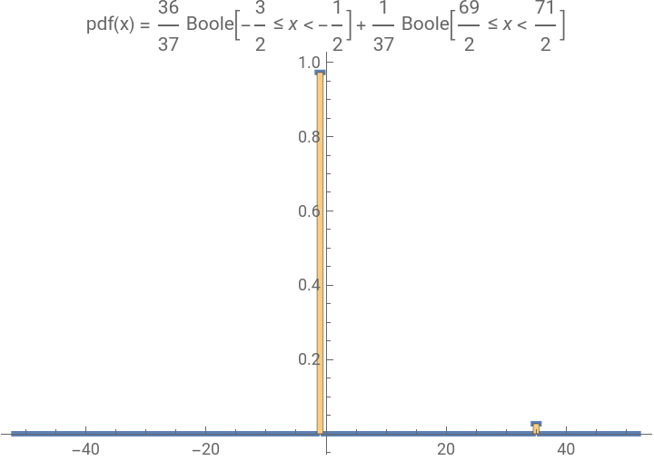
So it is the user’s job to fine-tune the start location (and far end location) and the bin width to get computational results (of mean and variance) which come close to the true results. I get reasonably close with the bin spec .
-,,1
3
2
73
2
In[]:=
bspec=-,,1;(*try{50}{25}{1}then-,,1*)hD=HistogramDistribution[data,bspec];Show[Plot[PDF[hD,x],{x,-52,52},PlotLabelRow[{"pdf(x) = ",PDF[hD,x]}],PlotStyleAbsoluteThickness[3]],Histogram[data,bspec,"PDF"]]{PDF[hD,x],Mean[hD],N@Variance[hD]}
3
2
73
2
3
2
73
2
Out[]=
Out[]=
Boole-≤x<-+Boole≤x<,-,34.1637
36
37
3
2
1
2
1
37
69
2
71
2
1
37
In[]:=
PDF[,x]
Out[]=
36
37
1
37
So why bother with HistogramDistribution[], if for a finite list of values the calculation of mean, expectation, variance, etc will always be off (wrong) compared to quantities computed from EmipiricalDistribution[] of the identical list of values?
Good question. The only answer i have is: The pdf of the histogram distribution is continuous (thus, can be integrated, if needed) and its Plot[] is meaningful, whereas the pdf of the empirical distribution is “impossible” to plot unless you resort to DiscretePlot[] but even then you can’t really interpret much from its plot because the discrete plot might be missing points.
Good question. The only answer i have is: The pdf of the histogram distribution is continuous (thus, can be integrated, if needed) and its Plot[] is meaningful, whereas the pdf of the empirical distribution is “impossible” to plot unless you resort to DiscretePlot[] but even then you can’t really interpret much from its plot because the discrete plot might be missing points.
Conclusion:
If you need to compute a statistic with high accuracy from a list of values, better do it with empirical distribution. If you need to display how a list of values is distributed over its range, do it with Histogram[] and optimize the bin width specification. Plotting the pdf of HistogramDistribution[] plots the roof of the histogram. For what would you need that?
If you need to compute a statistic with high accuracy from a list of values, better do it with empirical distribution. If you need to display how a list of values is distributed over its range, do it with Histogram[] and optimize the bin width specification. Plotting the pdf of HistogramDistribution[] plots the roof of the histogram. For what would you need that?
Hiermit sei die Aufgabe hinreichend bearbeitet.