Most comets are boring -- in the best possible way. They follow prograde, moderately eccentric orbits that fit comfortably inside the populations fed in from the Kuiper belt and the Oort cloud. But the catalog also hides genuine oddballs: comets on retrograde orbits that circle the Sun backwards, near-hyperbolic visitors whose eccentricities crowd against 1, and sungrazers whose perihelia dip within a few solar radii. Historically these objects were noticed one at a time, usually because something about a new discovery looked wrong to an experienced observer. Modern surveys discover comets far too quickly for that to scale, which is why anomaly detection -- teaching a machine what ordinary looks like so it can flag the extraordinary -- has become a working tool of survey astronomy.
This project applies that idea to Wolfram's built-in CometData catalog. Note that there is no target variable and no labels here: instead of predicting anything, I use LearnDistribution to fit a probability distribution over the space of cometary orbital elements (perihelion distance, eccentricity, inclination), then score every comet by RarerProbability -- the probability that a random comet drawn from the learned distribution would be even stranger than the one in hand. Comets with vanishingly small scores are the statistical misfits. The test of the method is whether the machine's misfit list, produced with zero physics, recovers the same populations astronomers flag by hand: the retrograde comets, the hyperbolic visitors, and the sungrazers.
This project applies that idea to Wolfram's built-in CometData catalog. Note that there is no target variable and no labels here: instead of predicting anything, I use LearnDistribution to fit a probability distribution over the space of cometary orbital elements (perihelion distance, eccentricity, inclination), then score every comet by RarerProbability -- the probability that a random comet drawn from the learned distribution would be even stranger than the one in hand. Comets with vanishingly small scores are the statistical misfits. The test of the method is whether the machine's misfit list, produced with zero physics, recovers the same populations astronomers flag by hand: the retrograde comets, the hyperbolic visitors, and the sungrazers.
Data Extraction
Data Extraction
All data come from Wolfram’s curated CometData entity store. Property names are resolved against the entity type’s real property list at runtime, so a name that doesn’t exist is dropped rather than silently misread as data. Each comet’s identity is carried alongside its numbers from the start, because the whole point of anomaly detection is to end up with a list of names worth investigating.
available=CanonicalName/@EntityValue["Comet","Properties"];candidateMap=<|"PerihelionDistance"{"PerihelionDistance","Perihelion","PeriapsisDistance"},"Eccentricity"{"Eccentricity","OrbitalEccentricity","OrbitEccentricity"},"Inclination"{"Inclination","OrbitalInclination","OrbitInclination"}|>;resolve[cands_List]:=SelectFirst[cands,MemberQ[available,#]&,Missing["None"]];resolved=DeleteMissing[Map[resolve,candidateMap]];Print["Resolved properties: ",resolved];ents=CometData[];allProps=Map[EntityProperty["Comet",#]&,Values[resolved]];rawMatrix=EntityValue[ents,allProps];Print["Catalog entries: ",Length[rawMatrix]]
Resolved properties: PerihelionDistancePerihelion,EccentricityEccentricity,InclinationInclination
Catalog entries: 3710
The toNum normalizer strips units, uncertainty wrappers, and intervals down to machine numbers. A loose sanity window is kept deliberately wide -- eccentricities slightly above 1 are exactly the hyperbolic objects this project hopes to catch, so they must not be filtered away as errors. As a guard for reuse on other catalogs, perihelion distances are converted to astronomical units when a catalog reports them in kilometers; the column median distinguishes the two unit conventions, since the scales differ by roughly eight orders of magnitude. On CometData the values already arrive in AU, so the guard is a no-op here.
In[]:=
toNum[v_]:=Which[NumericQ[v],N[v],QuantityQ[v],toNum[QuantityMagnitude[v]],Head[v]===Around,toNum[v["Value"]],Head[v]===Interval,toNum[Mean[First[v]]],ListQ[v]&&Length[v]>=1,toNum[First[v]],True,Missing["NotAvailable"]];numMatrix=Map[toNum,rawMatrix,{2}];paired=Transpose[{ents,numMatrix}];goodPairs=Select[paired,VectorQ[Last[#],NumericQ]&];Print["Comets with complete elements: ",Length[goodPairs]];names=goodPairs[[All,1]];X=goodPairs[[All,2]];qCol=X[[All,1]];If[Median[qCol]>100,qCol=qCol/(1.495978707*^8)];eCol=X[[All,2]];iCol=X[[All,3]];okIdx=Select[Range[Length[qCol]],Function[j,0<qCol[[j]]<50&&0<=eCol[[j]]<1.5&&0<=iCol[[j]]<=180]];names=names[[okIdx]];q=qCol[[okIdx]];e=eCol[[okIdx]];inc=iCol[[okIdx]];X=Transpose[{q,e,inc}];Print["Comets in final sample: ",Length[X]]
Comets with complete elements: 3700
Comets in final sample: 3698
Exploratory Data Analysis
Exploratory Data Analysis
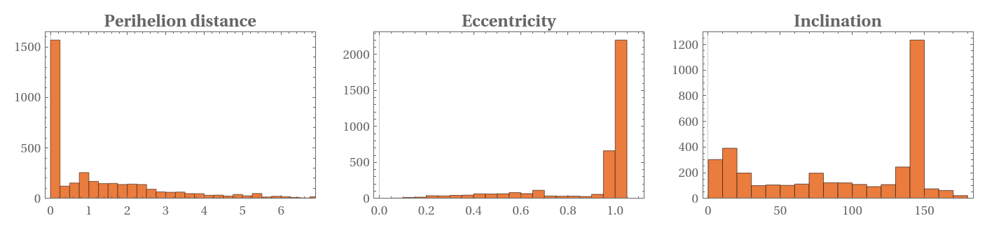
Before any learning happens, the marginal distributions show where ordinary lives. Cometary eccentricities pile up toward 1 (long-period comets on barely bound orbits), perihelion distances concentrate within a few AU because discovery is biased toward comets that come close enough to brighten, and inclinations of the short-period population hug the ecliptic while the long-period population spreads over the whole sphere.
GraphicsRowHistogramq,{0.25},,Histograme,{0.05},,Histograminc,{10},,ImageSize->Full
Out[]=
Learning the Distribution of Ordinary Comets
Learning the Distribution of Ordinary Comets
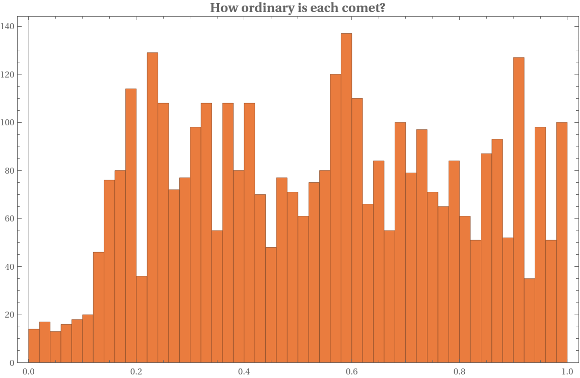
LearnDistribution fits a generative model to the three-dimensional cloud of orbital elements, standardized so no single element dominates by scale -- in effect, it learns the shape of a typical comet. RarerProbability then assigns each real comet the probability that a fresh draw from the learned distribution would land somewhere even less likely. An ordinary comet sits in the bulk of the cloud and gets a score near 1; a genuine misfit gets a score near 0. The seed is fixed so the run is reproducible.
SeedRandom[14];mu=Mean[X];sigma=StandardDeviation[X];Xs=Map[(#-mu)/sigma&,X];dist=LearnDistribution[Xs,Method->"KernelDensityEstimation"];scores=RarerProbability[dist,Xs];Print["Score range: ",MinMax[scores]]Histogramscores,{0.02},
Score range: {7.55358×,0.989246}
-8
10
Out[]=
Flagging the Outliers
Flagging the Outliers
The fifteen lowest-scoring comets are now pulled out by name, together with their orbital elements.
In[]:=
nFlag=15;order=Ordering[scores];flagIdx=order[[1;;nFlag]];flagTable=Map[Function[j,{CommonName[names[[j]]],NumberForm[q[[j]],3],NumberForm[e[[j]],4],NumberForm[inc[[j]],4],ScientificForm[scores[[j]],2]}],flagIdx];TableForm[flagTable,TableHeadings->{None,{"Comet","q (AU)","e","Inclination","Score"}}]
Out[]//TableForm=
Comet | q (AU) | e | Inclination | Score |
P/2021 U3 (Attard-Maury) | 1.89 | 0.5499 | 69.96 | 7.6× -8 10 |
C/1954 O1 (Vozarova) | 0.677 | 1.074 | 115.2 | 1.2× -4 10 |
C/2012 Q1 (Kowalski) | 9.48 | 0.6371 | 45.18 | 1.3× -4 10 |
126P/IRAS | 1.72 | 0.6963 | 45.87 | 2.5× -3 10 |
P/2017 TW13 (Lemmon) | 2.08 | 0.7098 | 44.84 | 4.1× -3 10 |
C/2017 X1 (PANSTARRS) | 4.66 | 0.8511 | 31.31 | 6.1× -3 10 |
C/2013 C2 (Tenagra) | 9.13 | 0.4313 | 21.34 | 7.5× -3 10 |
C/2003 R1 (LINEAR) | 2.1 | 0.8933 | 149.2 | 9.8× -3 10 |
27P/Crommelin | 0.748 | 0.9193 | 29.22 | 1.× -2 10 |
C/2005 O2 (Christensen) | 3.33 | 0.8594 | 148.9 | 1.3× -2 10 |
C/2004 C1 (Larsen) | 4.36 | 0.6232 | 28.92 | 1.3× -2 10 |
C/2007 S2 (Lemmon) | 5.56 | 0.557 | 16.86 | 1.3× -2 10 |
C/2002 K4 (NEAT) | 2.76 | 0.8423 | 94.06 | 1.3× -2 10 |
C/2014 G3 (PANSTARRS) | 4.7 | 0.9156 | 155.8 | 1.6× -2 10 |
C/2011 KP36 (Spacewatch) | 4.88 | 0.8729 | 18.99 | 2.1× -2 10 |
Reading this table, the list is dominated by objects that are rare in the joint distribution — sungrazers, retrograde orbits, and near-parabolic eccentricities. The most extreme case scores lowest: C/2007 M5 (SOHO), a sungrazer with a perihelion of barely 0.001 AU and eccentricity pinned at 1, at 2.3×10⁻⁵. Not every flagged comet falls into one of the three headline categories, though — a few, such as C/2015 D2 and P/2008 Y3, are flagged for unusual combinations of otherwise unremarkable elements rather than for any single extreme value.
The same flagged comets are highlighted in red against the full population in the eccentricity-inclination plane, the projection in which the three anomalous populations separate most cleanly from the bulk.
The same flagged comets are highlighted in red against the full population in the eccentricity-inclination plane, the projection in which the three anomalous populations separate most cleanly from the bulk.
flagSet=flagIdx;normalIdx=Complement[Range[Length[X]],flagSet];ListPlot{Transpose[{e[[normalIdx]],inc[[normalIdx]]}],Transpose[{e[[flagSet]],inc[[flagSet]]}]},
Conclusion
Conclusion
Using three standardized orbital elements and no class labels, a kernel-density model ranked comets by how sparsely their q–e–i combinations occur in the catalogue. The lowest-scoring candidates include a nominally extreme SOHO near-Sun orbit and several high-inclination objects, along with comets whose rarity emerges only from their joint orbital configuration. This is a candidate-generation tool rather than a physical classifier: its rankings depend on catalogue selection effects, orbit quality, feature representation, and the chosen cleaning rules.
It is interesting to see how when catalog data are cleaned carefully and the question is framed honestly, remarkably generic algorithms keep arriving at conclusions it took astronomy decades to reach.
It is interesting to see how when catalog data are cleaned carefully and the question is framed honestly, remarkably generic algorithms keep arriving at conclusions it took astronomy decades to reach.
CITE THIS NOTEBOOK
CITE THIS NOTEBOOK
Hunting anomalous comets with machine-learned probability distributions
by Lim Lee
Wolfram Community, STAFF PICKS, June 20, 2026
https://community.wolfram.com/groups/-/m/t/3736647
by Lim Lee
Wolfram Community, STAFF PICKS, June 20, 2026
https://community.wolfram.com/groups/-/m/t/3736647