Genomic comparisons
Genomic comparisons
I will start with a list of GenBank accession IDs. These were culled from a large list comprised of sequences I have seen in recent literature, blogs, and elsewhere, all for the purpose of comparison to 2019-nCoV. GenBank has the data for these in FASTA format. The last two lines are comprised of IDs for several of the 2019-nCoV sequences that have been placed in GenBank to date. The first of those is the initial such.
In[]:=
manyviruses={"MG772933","MG772934","MK211376","KJ473816","KY417145","KF294455","KY417144","AY395003","AY394996","AY390556","EU371564","AY394985","EU371559","AY559093","NC_004718","AY304488","AY502927","GU553365","EU371562","AY278488","AY274119","NC_005831","MF542265","KY983587","KY967357","AY729016","NC_006579","NC_019843.3","NC_038294","MN908947.3","MN938384","MN975262","MN985325","MN988713","MN988668","MN994467","MN994468","MN997409","MN988669","MN996527","MN996528","MN996529","MN996530","MN996531"};manyviruses//Length
Out[]=
44
Importing sequences from GenBank
Importing sequences from GenBank
We obtain the sequences using a really handy function from the Wolfram Function Repository (WFR): ImportFASTA. It was written by my colleague Brendan Elli. It started out as code he wrote in response to a request I made in-house. No good deed goes unpunished. Also note that my colleague John Cassel has created a resource data object containing the 2019-nCoV examples above as well as new ones that have been more recently sequenced (he also provided some helpful advice for this notebook). For other useful resource of 2019-nCoV genetic data please see the following Wolfram Data Repository entry:
https://datarepository.wolframcloud.com/resources/Genetic-Sequences-for-Novel-Coronavirus-2019-nCoV-from-Wuhan-China
https://datarepository.wolframcloud.com/resources/Genetic-Sequences-for-Novel-Coronavirus-2019-nCoV-from-Wuhan-China
On my machine it takes around a second to obtain each sequence. From past usage I am fairly sure this has to do with server access requirements and not sequence lengths.
In[]:=
AbsoluteTiming[vseqs=Map[ResourceFunction["ImportFASTA"],manyviruses];]
Out[]=
{46.3862,Null}
We now separate out names and genome sequences. It turns out that some sequences have a trailing repeated “A” (for adenine) and others have this removed; in particular both types appear in the 2019-nCoV set, and this is almost certainly an artifact of either sequencing protocols or perhaps decisions to remove trailing “junk”. I found that by removing it uniformly we get results that seem not to suffer from artificial discrepancies.
In[]:=
names=vseqs[[All,1,1]];vstrings=vseqs[[All,2,1]];shortnames=Map[StringTake[#,30]&,names];vstrings=Map[StringReplace[#,"A"..~~EndOfString""]&,vstrings];
The lengths are all in the ballpark of 30K nucleotides, with the exception of two (they may have been only partial sequences).
In[]:=
Map[StringLength,vstrings]
Out[]=
{29776,29706,30256,29141,29694,21477,29754,29623,29659,29756,29508,29506,29727,29711,29727,29730,29727,29644,29598,29708,29727,27553,27246,27234,27202,14886,14885,30107,30099,29870,29838,29870,29870,29870,29869,29870,29870,29870,29869,29825,29870,29852,29854,29857}
Building a phylogenetic tree
Building a phylogenetic tree
Now we will create a phylogenetic tree, again with a handy WFR function, PhylogeneticTreePlot. I use a color scheme that is intended to group families but I do not claim to have done this without errors.
In[]:=
colors=Flatten[{ConstantArray[Brown,2],ConstantArray[Red,5],ConstantArray[Blue,14],ConstantArray[Green,4],ConstantArray[Cyan,4],ConstantArray[Black,15]}];stylednames=Thread[Style[shortnames,colors]];
In[]:=
ResourceFunction["PhylogeneticTreePlot"][vstrings,stylednames,AspectRatio1.5,ImageSize800]
Out[]=
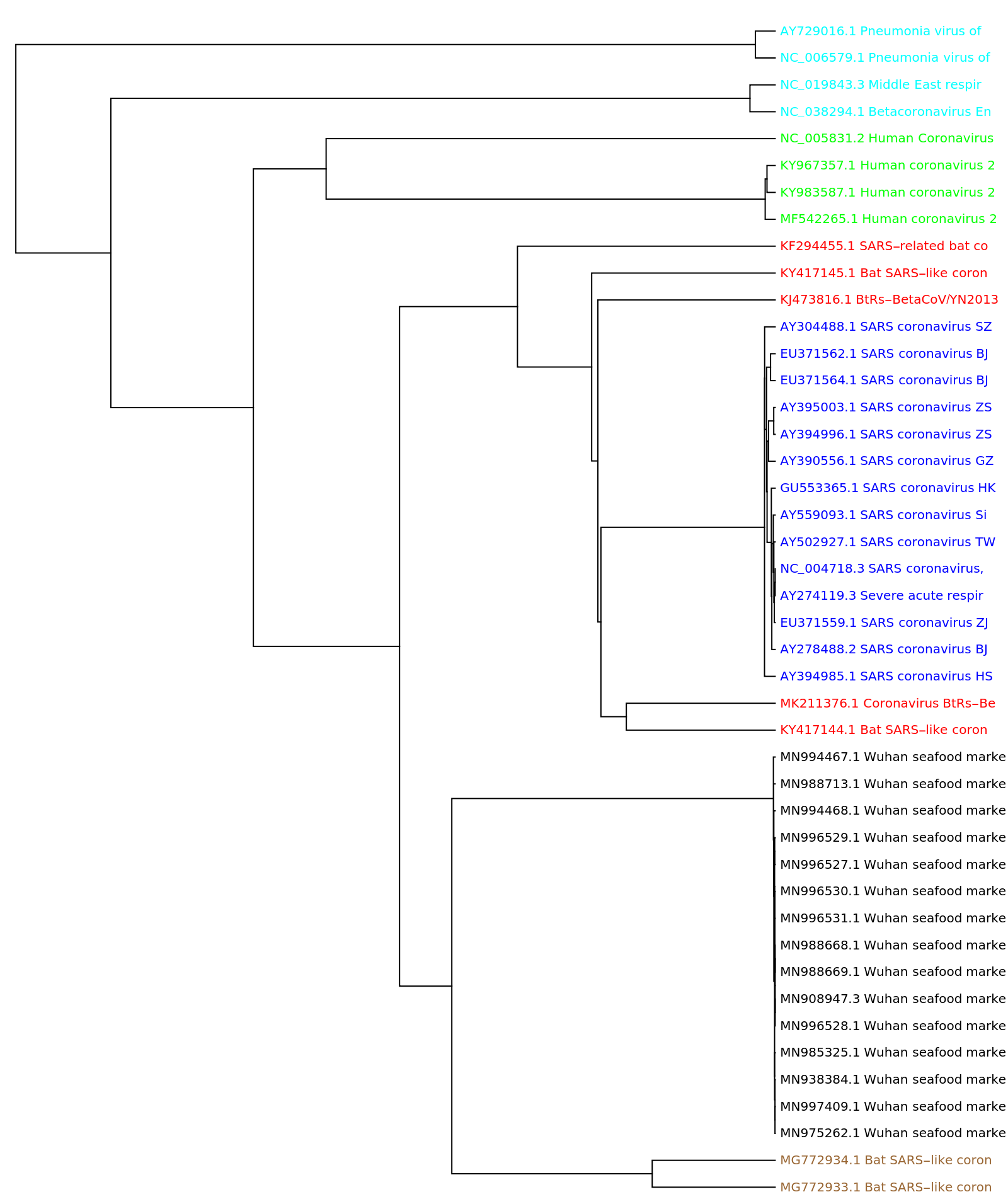
So no big surprises here. In particular this is in agreement with various analyses that have recently appeared, indicating that the 2019-nCoV has greatest similarity to the two bat SARS-like coronavirus with IDs MG772933 and MG772934 respectively.
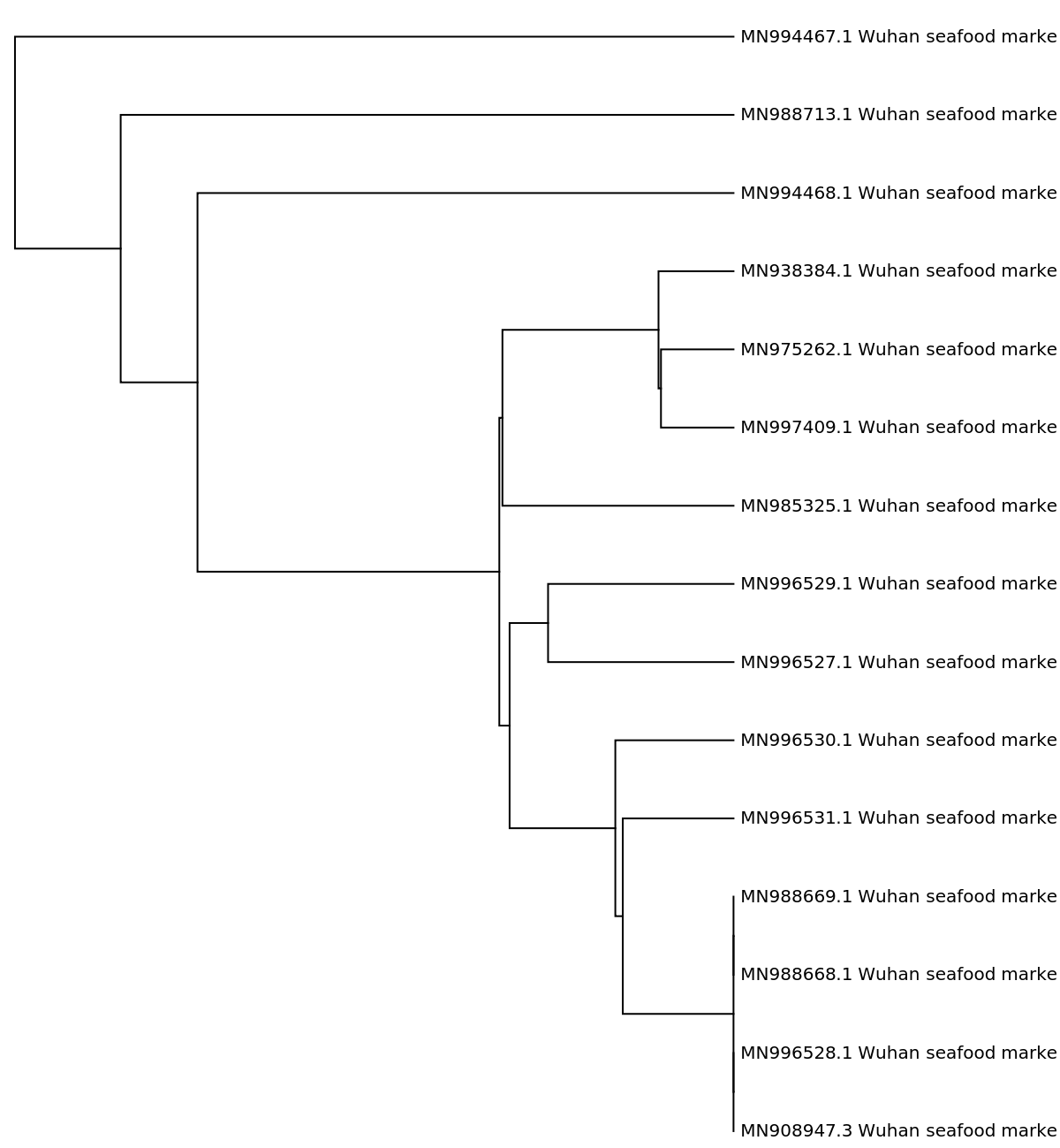
One can of course zoom in on, say, just the 2019-nCoV samples.
In[]:=
ResourceFunction["PhylogeneticTreePlot"][vstrings[[-15;;]],shortnames[[-15;;]],AspectRatio1.5,ImageSize600]
Out[]=
Illustrating in three dimensions
Illustrating in three dimensions
One can create numeric vectors from the genome sequences, and that is in fact what PhylogeneticTreePlot does behind the scenes. I will use essentially the same code as is in the definition notebook for that function, in order to provide a different illustration of the “distances” between these viruses. (For brevity I omit it here, but see last section.) One can access the code in question by opening the definition notebook with the code below.
In[]:=
ResourceObject["PhylogeneticTreePlot"]["DefinitionNotebook"]
Out[]=
NotebookObject

Using this code I created a set of numeric vectors, each of length 40, for the genome sequences. They are stored a vecs2019nCoV and for convenience of data exploration I include them below.
Out[]=
Now we can use dimension reduction to place these in three dimensions, in a way that attempts to retain approximate distances between all pairs (this is the point of dimension reduction).
styled=Apply[Style,Thread[{DimensionReduce[vecsCOV,3,Method"LatentSemanticAnalysis"],colors}],{1}];ListPointPlot3D[styled,PlotRangeAll]
The (clustered) two brown points, as expected, are closest to the black 2019-nCoV cluster. the “TSNE” method shows a somewhat different picture however.
I am somewhat partial to a method not built into DimensionReduce, known as Multidimensional Scaling. So partial, in fact, that I put it into the WFR.
This gave a plot that is not too different from the latent semantic analysis method. The Properties and Relations section of the definition notebook gives an indication of why they are similar (in brief: both are based on the Singular Values Decomposition from linear algebra).
Locating possible “hot spots” on a genome sequence
Locating possible “hot spots” on a genome sequence
This section is, uhm, on the “tentative” side. I simply lack the genetics background to assert that the following analysis carries much meaning from a biological point of view. But it does show tools that can be deployed regardless. (Strictly speaking, I also am lacking in genetic expertise for the preceding genome comparison section, but there at least I have the benefit of having developed tools and tested them on several benchmark data sets.)
The idea we pursue is as follows. It is known that coding sections (exons) of genomes correlate heavily with a periodicity of three. Of course this forces the question of how to gauge periodicity. It turns out that several methods are available for this purpose. I will show two, and we will see that they are in rough agreement. It should be noted that these are crude and, at best, accurate to tens of nucleotides. With emphasis on “at best”. For both methods we need to form a signal from a genome sequence. One method is fairly well known and allows us to apply basic Fourier methods to get a frequency, from which we can then derive a period. Of course there can be multiple large frequencies, and corresponding periodicities. But the length three period, when it appears, is dominant, and we will use that to advantage.
We illustrate with the first of the 2019-nCoV genomes in our list.
In order to localize “hot” areas (that is, regions that show the three-periodicity), we will segment into overlapping substrings of length 500, with a spacing of 100. When we locate substrings of interest we will merge any that have centers falling strictly within the range of prior substrings of interest.
Method 1: construct sequences in 3D and compute the Fourier spectra
Method 1: construct sequences in 3D and compute the Fourier spectra
The idea is to regard each of the four nucleotides as occupying a vertex of a regular tetrahedron centered at the origin. So each gets associated to a point in 3-space. The array of three dimensional values thus created can then be analyzed for frequency information using Fourier.
We get the three Fourier sequences for each of these substrings.
Now sum absolute values for the three sequences (one per dimension) obtained from each substring. We remove the first components to avoid an artificially high DC component.
The code below will “clump” these into longer runs, when later middle points fall inside prior intervals.
Method 2: Irregular periodograms find common gap frequencies
Method 2: Irregular periodograms find common gap frequencies
Here again we use a WFR function, this one being IrregularPeriodogram. I follow an example in the documentation for that function, so again I include the line for opening the definition notebook/
The idea is to find locations of certain dinucleotides, specifically “AA”, ”AT”, and ”TT”. There is a large body of literature indicating that these in particular show three-periodicity. Actually one usually works with related trimers or tetramers, but the relatively small substring lengths warrant using the dinucleotides to get sufficient data. We work with gap lengths between these dinucleotides, and try to assess strong frequencies from that data. The three-periodic substrings will appear as having strong frequency components at 2π/3 and 4π/3. To cut back on noise in assessing common gaps, we remove those that only appear one time in a given substring.
Now compute periodograms based on these gaps. Note that while we compute these at regular intervals, the inputs are not regular and so the irregular periodogram really is warranted. We compute over a range that begins well before 2π/3 so that we can remove any that might be large near that value but have larger spikes earlier.
Again it is instructive to see some plots.
We will determine candidates
Several show strong spikes in the frequency range of interest, and they tend to exceed 150. We use that to determine the “keepers”.
Again we clump these.
This tends to be a more spare list than that from method 1. All the same, they do appear to have considerable overlap.
Alignment-free alignment
Alignment-free alignment
Genome alignment is done in order to either connect subsequences, or to compare one genome to another to check for possible relationships. It is typically performed using string processing based methods, and these can be expensive. In this section i will show a method that falls very much within the “alignment-free” family of genome analysis. But we deploy it in a way that actually can inform alignment possibilities, by narrowing the search ranges.
The idea is as follows. From the phylogenetic tree in the first section we already know that the 2019-nCoV appears to be most closely related to two bat SARS-like coronaviruses. We will compare the same 2019-nCoV genome used in the prior section to one of those two similar ones. As in the last section we again use substrings of length 500. For this work I do require the code used in the WFR function PhylogeneticTreePlot, so this will be a bit more elaborate from the code point of view. One of the tools is itself a WFR function, FCGRImage. That function actually creates images from DNA strings. Since we really want the underlying matrices we convert back using ImageData.
Support code
Support code
Application to our two genomes
Application to our two genomes
The method proceeds as follows. We preprocess both sets of substrings, first obtaining the FCGR arrays and then reducing dimension with the discrete Fourier Cosine Transform (using FourierDCT). The older genome is the “reference” set and the 2019-nCoV processed strings will be our “test” set. A next step is to take the reference processed vectors and further reduce dimension using the Singular Values Decomposition (SVD for short, implemented as a function called, not surprisingly, SingularValuesDecomposition). We return both a lookup function created using Nearest, and the right side conversion matrix from the SVD. this latter is needed in order to also reduce dimensions for the test vectors.
The processing from here is straightforward. Each text vector corresponds to a substring in the test genome sequence. We look up the “closest” dimension-reduced vector from the reference genome. Sections that tend to align well will be recognized because contiguous chunks in the test genome will have, as closest neighbors, approximately consecutive runs in the reference set.
I will defer on writing yet more code to do a detailed associating of consecutive runs from one to similar runs from the other. By eye one can observe that these initially seem to align quite well. We do see that fairly late in the set, vector 69 from the reference set is nearest neighbor to a few in the test set.
The first such is of course expected. The later ones indicate that there is something of a gap in the test set, where matches to the reference genome are out of alignment. We also see that there are a few matches to chunk 227, just before and after the final match to chunk 69. We’ll chek their locations.
This indicates that the sequences are not only approximately back in alignment, but that they seem to be so at the same positions in the respective genome sequences.
For those interested in the underlying method, the reference is:
D. L. Alignment-free genomic sequence comparison using FCGR and signal processing. BMC Bioinformatics 20:742 (2019). DOI: 10.1186/s12859-019-3330-3 (handy link)
D. L. Alignment-free genomic sequence comparison using FCGR and signal processing. BMC Bioinformatics 20:742 (2019). DOI: 10.1186/s12859-019-3330-3 (handy link)
Final remarks
Final remarks
I showed a few tools of the in Mathematica and the Wolfram Function Repository that one can use for genome analysis. These were applied to timely examples from the recent 2019 novel coronavirus. As should be obvious, I focused, perhaps to a shameless extent, on methodologies with which I am quite familiar. I hope these are applicable to work other people are doing. I also hope others will consider contributing their own work to this forum and, if applicable, to the WFR.