Organisms in nature must adapt to environments that change over time, whether cyclically or irregularly. This work uses cellular automata (CA) as a minimal model of biological organisms to study how simple discrete systems adapt to changing environmental demands, following Stephen Wolfram’s Evolution Model. CA rules serve as the organisms’s genotype, and its resulting pattern as phenotype. The target fitness values represent the environmental demands that switch between two states over time. Across 100 independent CA runs of 4800 steps each, we find that CA populations exposed to periodic, cyclic environments show a clear evolutionary learning curve. Namely, the delta between the target and realised fitness decreases monotonically and confidence intervals across replicate runs narrow over time, showing adaptation and robustness. When the environmental changes irregularly, the improvement in adaptation is no longer monotonic, but CAs still show some signs of improvement in later iterates. Finally, we test for anticipation, which is whether an organism’s current and future behaviour is shaped by its history, preparing it for future environmental changes. We find that this anticipation is sort of symmetric; CAs struggle to anticipate a harder environment after exposure to an easier one, while the reverse transition has a similar pattern. These results suggest that even minimal, simple organisms could have a memory using their environmental adaptation history that shapes their future behaviour.
Background
Background
Biological evolution gives us the change of organisms over time. Each organism lives in an environment, for example, a rainforest. Each environment has its own requirements posed to the organisms, such as, the need to blend into a forest environment to not stand out to predators. However, as natural and man-made challenges come to play, the environments of the organisms change. The organism must learn how to adapt. Those who cannot adapt, do not make it. From this, we have the idea of natural selection, or survival of the fittest, where organisms who are able to adapt survive the longest.
So what sort of changes happen to the organism as it adapts? What if the environment is cyclically changing, in periods of time? We start the organism in some environment A for an amount of time, then change to some environment B, and go back to A again. Can the organism adapt, does it adapt better the more cycles we have, and can it anticipate the environment is going to change? These thoughts also beg the question of whether the organism can adapt to irregular periods of environments.
To contribute to answering these questions, we need organisms simple enough so that we can run evolutions on them lots of times, and complex enough such that we can distinguish their “genotype” and “phenotype”. Stephen Wolfram’s recent work makes the case that cellular automata (CA, in this essay) are close to a minimal model for this task, where we think of the rules of the CA as its genotype, and its appearance after its run by a program as its phenotype. Mutations in organisms translate to state changes in the CA, and selection corresponds to keeping mutations that don’t decrease the fitness, and discarding ones that do. Taking Stephen Wolfram’s idea that simple rules lead to complex behaviours, we can use cellular automata as proxy for our organisms. Cellular automata have an initial condition and a rule which governs how they behave. They can be used to visualise and explain this adaptation as it happens through simple sets of rules.
Thus, our model effectively represents identity (genotype) and behaviour (phenotype) of organisms in a simple yet powerful way.
Model Set-Up
Model Set-Up
We now go into more depth about what cellular automata are and how we can use them to answer how evolution works under changing environments. Cellular automata are grids of cells that can take a finite number of states. The CA follows rules to update the cells after starting from an initial condition. The initial condition is simply a starting update rule and position. In our diagram below, we can see a rule plot on the left showing a visual representation of the rules by which the cells update, and on the right, the resulting cellular automaton after some timesteps.
Out[]=
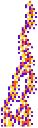
The cellular automata used in this study use 4 different states, and are thus more complex than elementary cellular automata. Not every type of CA is useful to us here. We are using automata rules (genotypes) that produce finite morphologies (phenotypes) because we can measure things on a finite organism. The primary fitness function we’re using is lifespan, and lifespan itself is a constraint on finite size. Hence, we are using finite CA in our experiments.
As previously stated, we consider our CA organisms to have their phenotype as physical characteristics of their appearance (like the octopus arm above), and their genotype as the rules and initial condition. The environment the CAs are placed in are represented by a target fitness value. For our study, we define target values for the cellular automata to meet, and these target values represent the demand of the environment at that time. We consider the length of the CA to be the fitness in the environments. In the diagram below, we show a target line in black, which starts with environment A at target length 10 for 200 steps, then goes to environment B at target length 60 for 200 steps, and the real adaption in red of a CA in the environments. An important thing to note at this time is that this is what we are considering as 1 cycle in the rest of the essay.
As previously stated, we consider our CA organisms to have their phenotype as physical characteristics of their appearance (like the octopus arm above), and their genotype as the rules and initial condition. The environment the CAs are placed in are represented by a target fitness value. For our study, we define target values for the cellular automata to meet, and these target values represent the demand of the environment at that time. We consider the length of the CA to be the fitness in the environments. In the diagram below, we show a target line in black, which starts with environment A at target length 10 for 200 steps, then goes to environment B at target length 60 for 200 steps, and the real adaption in red of a CA in the environments. An important thing to note at this time is that this is what we are considering as 1 cycle in the rest of the essay.
Out[]=
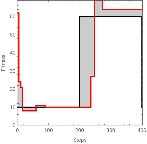


In the diagram above, we can see that there is a clear difference between the target fitness value and the real fitness value at some points (the difference indicated by the Grey filling). This difference gives us a metric for evaluating how well the CA can adapt to the given target environment values. Ideally, we would like to see that the CA minimises this metric over time. To properly evaluate the evolutionary dynamics, the methodology was to have 100 CA runs of 4800 steps each. This way, we get enough data on how the CAs evolve over time.
We first take a look at the fitness over time, then go into experiments for cyclic and irregular environments, before finally moving onto the anticipation capabilities of the CA.
We first take a look at the fitness over time, then go into experiments for cyclic and irregular environments, before finally moving onto the anticipation capabilities of the CA.
Evolutionary Dynamics of Cellular Automata
Evolutionary Dynamics of Cellular Automata
Given that the environment changes periodically, one way to visualise how the system adapts over time is to make the plot below (inspired by Stephen Wolfram’s writings), which illustrates a single CA run of our experiment (31/100). The red line plotted here represents the true raw fitness value. Its distinct rise and fall pattern throughout the 4800 steps shows the cyclicity of the CAs, which is likely driven by the periodic cycles in the environment. On the other hand, the black step plot tracks the historical best-so-far (or maximum) fitness at that timestep, which only moves upwards when an evolutionary milestone is reached. These milestones are referred to as breakthroughs. Each of the breakthrough points has an icon attached to it containing the phenotype of the CA at the time. As time goes on, you can see that these breakthrough steps begin to saturate, indicating that the CA reaches an evolutionary limit under the periodic environments.
Out[]=
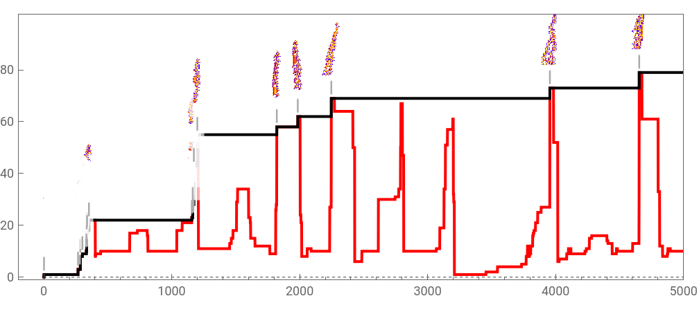


What is interesting in this graph is that the evolutionary dynamics reveal an increase in adaptability over time. In the early iterations (before step 1500), the CA struggles to quickly recover from environmental shifts and usually cannot make it back to the maximum fitness. In contrast, during the later iterations (so after 2000 steps), the red realised fitness line spikes quickly and is able to meet the black line (which is the historical maximum fitness), almost immediately after a cycle. This suggests that the evolution of the CA has selected rules that are robust and capable of adapting well to the periodic environment.
Cyclic Environments
Cyclic Environments
Starting with exploring cyclic, periodic environments, which can be considered better predictable, we look at the phenotypes at different stages of the evolution, and compute an adaptation metric which will give us more information about how well the CA organisms are able to adapt. We would expect that the organisms can adapt to these cyclic environments fairly easily, since we have cycles everywhere in nature (day-night, seasons, tides).
Out[]=

The plot above shows how the phenotype of the organism changes through evolutionary time in this periodically changing environment, alluding to a clear adaptation back and forth into the two environments. We can see that the length of the phenotypes appears to changes periodically. Then, we can focus our attention in the ‘transitional’ period of the environmental switch, which reveals how fast can the phenotype change at the transition. The left plot indicates the phenotypes in the first cycle, where the right plot indicates the phenotypes in the last cycle.
Out[]=
Steps 1–401
Steps 4401–4801
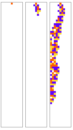
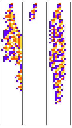
Note that we have 12 cycles in total in 4800 steps. Both of these plots evidence that cellular automata as simple organisms can adapt to cyclic environments. The question moves towards how well can they adapt, and how long it takes for them to adapt. For this, we compute the absolute difference between the target environment fitness values, and the real average evolution fitness values from the 100 runs for every cycle.
Computing the Delta of Fitness Over 4800 Steps
Computing the Delta of Fitness Over 4800 Steps
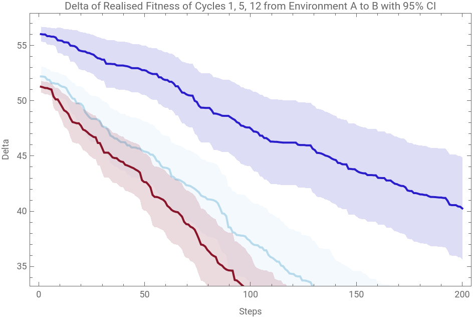
Below we see the delta of the realised fitness for each of the 12 cycles. The graphs below tell us the absolute difference between the target fitness and the actual fitness on average of the 100 CA runs for each of the 12 cycles. Note that while a cycle is typically 400 steps in total, our curves are plotted between 0 and 200 steps. This is because we are interested in the time to adaptation starting from the first environment, and going to the second environment. So, we only consider the realised fitness in steps 200-400 of a cycle. In the plots below, there is a clear monotonically decreasing pattern, and as we iterate over the cycles, we see that the delta curve becomes more steep. This signals to us that the realised fitness and adaptation to the target fitness improve with predictable environments.
Out[]=
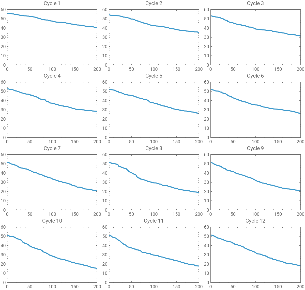
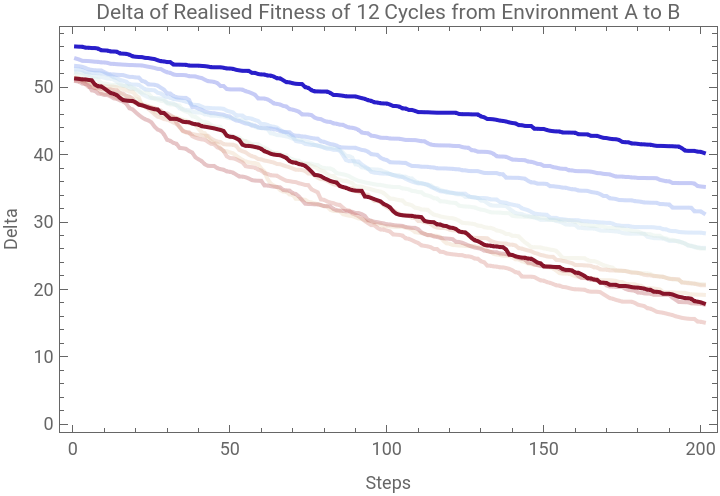
Upon making a superimposed graph of the deltas for each cycle, with a warmer colour code corresponding to increasing cycles, what is striking here is the difference between the deltas in the first cycle and in the last cycle. These results tell us that the CAs are indeed adapting better with more cycles.
Out[]=


A notable factor here is that at around cycle 9, the adaptability does not strictly increase anymore and it might indeed recede a bit. Across many replicates, these adaptive patterns are robust, as shown here by the confidence intervals from 100 independent runs. On a side note, we see a very beautiful waterfall.
Out[]=
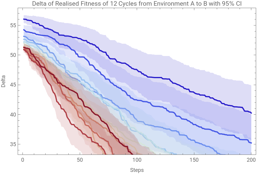


When taking an even closer look at the initial, middle, and end points of these environmental cycles, we see that the confidence interval narrows over cycles, meaning that our measurements become more precise. This implies that the 100 runs behave more similarly to one another as timesteps progress.
Out[]=
Irregular Environments
Irregular Environments
So far, we have explored adaptation in cyclic, periodic environments. We showed that organisms are readily adaptable and that they show a kind of ‘evolutionary learning’ when exposed to more and more such cycles. However, one might wonder whether this pattern persist when the environment is not as predictable. Ultimately, one might think that the previous cycles are not very different than a non-changing environment, in the sense that one could know beforehand what would be the fitness constraint in any future time step. What if this was not the case?
To test this, we made sure to have a maximum of 2.4k steps allocated to each environment (for a total of 2 environments in 4.8k steps), with periods of 100-300 steps following a bell curve with a mean of 200 steps. This resulted in 14 irregular ‘cycles’ or iterates. Below, we can see the evolution of phenotypes of cellular automata in this set-up.
To test this, we made sure to have a maximum of 2.4k steps allocated to each environment (for a total of 2 environments in 4.8k steps), with periods of 100-300 steps following a bell curve with a mean of 200 steps. This resulted in 14 irregular ‘cycles’ or iterates. Below, we can see the evolution of phenotypes of cellular automata in this set-up.
At the beginning, it does not seem to be as adaptive as the cyclic environments. As we did with the cyclic environments, we again plot a realised fitness delta going from target length 10 to target length 60 for each irregular iterate to see the adaptive performance.
These results clearly do not show the monotonically decreasing delta type of adaptive ‘learning’ we had in the previous experiment. However, these curves do not seem entirely random, either. There seems to be a dip in the middle of the curve for the first iterate, and this dip presents itself later in the higher cycles. The last iterate, 14, appears as an anomalous graph in this superimposed plot. The valley in the middle is also not too noticeable. Why is it that we sort of trail off from the general idea with the last two cycles? And why does the valley change position with a higher amount of iterates?
While early iterates (represented by the cooler colours) successfully adapt to the environmental changes in the first few steps and struggle in the last few steps, the plot does show that the delta of realised fitness does decrease over the cycles, seen by the plots of iterate 13 and 14. Since the periodic environments are irregular and do not have a fixed number of steps, the run lengths can vary significantly, providing a reason why iterate 13 and 14 appear to be significantly shorter than the rest of the plots. However, this also causes some problems in the interpretation of the plots. Due to the fact that iterate 14 was so short and the cellular automata had ran for a significant amount of steps, this could lead to slightly misleading results of the delta fitness values.
The shifting of the valleys’ positions could be attributed to the improved adaptation of the CAs over time. This is because over timesteps and iterates, we see that the ‘valley’ shape appears later, and additionally we see less of a valley, and hence also less of a rebound. This means that the CAs learn to adapt better to the irregular environments over iterations and timesteps, even though it still does not reach the monotonically decreasing state as with the cyclic experiments.
To take a closer look into the curves, below we find the plots for the initial, middle, and end iterates for the irregular periods. Unexpectedly, the first cycle has the same amount of variation in its values for the delta of realised fitness as the last cycle, meaning that the measurements do not improve in precision. Particularly with iterate 11, we see that it has very wide confidence intervals towards the end, meaning that the values for the 100 runs are imprecise over time.
Anticipation
Anticipation
Anticipation is an important factor to check in our evolutionary experiments because it gives us an idea of whether simple organisms that we represent by cellular automata could anticipate the next environment based on their history and current environment. This constitutes the memory of the organism as it evolves. Past experiences shape what organisms can do, and shape what organisms will do. The following plots give us an idea of how anticipation works with our simple CA organisms.
The plot below gives us the graphs of the metric of whether the organism can anticipate environment B (of target value 60) while being in environment A (of target value 10). Since the delta of realised fitness is monotonically increasing over time, and is steeper for higher cycles, this indicates that the organisms have a difficult time going from an easier environment to a harder environment. They can adapt well to the regular cycles, but then the more they are adapting and are familiar with the cyclic periodic environment changes, they struggle to anticipate a tougher environment. This results in the higher delta across cycles. This finding seems to make some intuitive sense; when we reflect on our own routines in life, we notice that its harder for us to make a sudden change.
The plot below gives us the graphs of the metric of whether the organism can anticipate environment B (of target value 60) while being in environment A (of target value 10). Since the delta of realised fitness is monotonically increasing over time, and is steeper for higher cycles, this indicates that the organisms have a difficult time going from an easier environment to a harder environment. They can adapt well to the regular cycles, but then the more they are adapting and are familiar with the cyclic periodic environment changes, they struggle to anticipate a tougher environment. This results in the higher delta across cycles. This finding seems to make some intuitive sense; when we reflect on our own routines in life, we notice that its harder for us to make a sudden change.
On the other hand, we have the plot below for whether the organism can anticipate environment A while being in environment B. The result of the plot is asymmetric to the plot above. Why is there a spike at the beginning? And why are the delta values for this plot higher on average than for the previous one?
The spike at the beginning of the graphs decreases with each cycle iteration, causing the curves to shift downwards (once again, the warmer curves represent a higher cycle). This plot captures well how the CA anticipates the easier environment A while still confined to the demands of the tougher environment B. Each curve rises sharply at the start because the organism is still carrying environment B’s phenotype into the new cycle before it catches up to the phenotype of A. The size and steepness of this rise decreases over the cycles, with cycle 12 rising much less before flattening. The shrinking suggests that the CA anticipates the downshift to A more efficiently, needing less time to prepare for the easier environment.
This is still consistent with our intuition, which would be that its easier to move from a tougher environment into an easier one. We also can see that the CAs are overshooting a bit since the delta values are higher on average compared to the last plot. This also makes sense because they want to be prepared when the environment becomes tougher again.
Discussion
Discussion
This essay used cellular automata as a minimal model to investigate whether simple organisms can develop something like memory and anticipation purely through interacting with a cyclic or irregular environment. Across our experiments, the answers were intuitive, and were a yes for cyclic environments. In the cyclic environments, the CA populations showed a clear evolutionary learning curve, adapting faster and more reliably with each cycle. This improvement was not as stark for irregular environments, but was still present, suggesting that the CAs do find a way to try adapt to the changing environments. From the anticipation experiments, we could see that the CAs anticipated both shifts from the tougher environment to the easier and vice versa. This tells us that the CA’s rule set carries a part of its evolutionary history that shapes its behaviour before the environment changes.
These results allude to an old tension in how we think about causality in physical versus living systems. Classical dynamics treats a system’s present state as governed only by its past, where behaviour is entirely reactive and there is no dependency on the future to shape the current state. The simple organisms we simulated here complicate this; since we observe some markers of anticipation. We observe what Robert Rosen describes as anticipation, where a system’s current behaviour is based on the future environment which it has not yet experienced, but it uses its experience from past environments and evolutionary history.
More broadly, we can interpret that anticipation does not require complex biological systems, but rather a system that can encode information about itself, like its evolutionary history (containing selection, and environmental structure). Given this history, the CA can have an expectation about the future that it uses as an anticipation. Lots of open questions remain after this project. Since we only had two environments, and a relatively simple fitness function, it would be worth investigating the topic of investigation in more depth. We plan to study more complex environmental cycles, the limits of ‘evolutionary memory’, and which conditions lead to anticipatory behaviour.
Acknowledgements
Acknowledgements
First and foremost, I would like to extend my greatest thanks to my mentor, Pedro Márquez-Zacarías. He provided amazing guidance throughout the project and always had novel “side quests” for me to look further into. Whenever I pitched an idea, he was always willing to help me make it into something concrete to include in the project. Then, I would like to thank Dr. Stephen Wolfram for the main idea of this project. Finally, I want to say a huge thank you to everyone who I became friends with during the program; they all contributed to the fantastic experience I had.
References
References
1
.Wolfram, S. (2024, May 3). Why does biological evolution work? A minimal model for biological evolution and other adaptive processes. Stephen Wolfram Writings. https://writings.stephenwolfram.com/2024/05/why-does-biological-evolution-work-a-minimal-model-for-biological-evolution-and-other-adaptive-processes/
2
.Wolfram, S. (2025, November 11). What’s special about life? Bulk orchestration and the rulial ensemble in biology and beyond. Stephen Wolfram Writings. https://writings.stephenwolfram.com/2025/11/whats-special-about-life-bulk-orchestration-and-the-rulial-ensemble-in-biology-and-beyond/
3
.Wolfram, S. (2024, December 5). Foundations of biological evolution: More results & more surprises. Stephen Wolfram Writings. https://writings.stephenwolfram.com/2024/12/foundations-of-biological-evolution-more-results-more-surprises/
4
.Bernhardt JR, O’Connor MI, Sunday JM, Gonzalez A. 2020 Life in fluctuating environments. Phil. Trans. R. Soc. B
5
.Rosen, R. (2012). Anticipatory systems: Philosophical, mathematical, and methodological foundations (2nd ed.). Springer. https://doi.org/10.1007/978-1-4614-1269-4
AI Disclosure
AI Disclosure
The following generative AI tool was used in this project: Claude Sonnet 5. It was used for debugging code in the particularly dense parts and finding obscure functions that do just the right thing. All code and written content was reviewed, understood and approved by the author.
CITE THIS NOTEBOOK
CITE THIS NOTEBOOK
Evolutionary Dynamics in Changing Environments
by Anusha Asthana
Wolfram Community, STAFF PICKS, July 16, 2026
https://community.wolfram.com/groups/-/m/t/3763024
by Anusha Asthana
Wolfram Community, STAFF PICKS, July 16, 2026
https://community.wolfram.com/groups/-/m/t/3763024