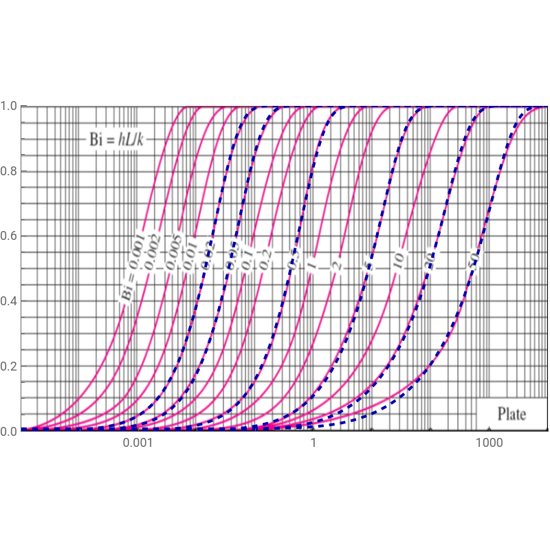
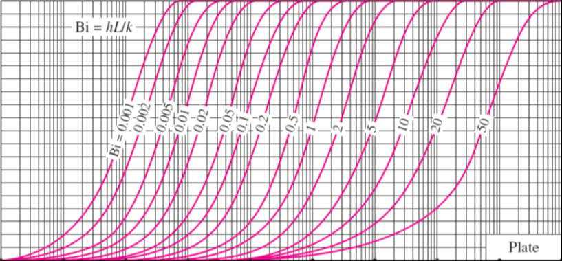
This notebook reproduces the Gröber chart for a large plane wall of thickness , as presented in the transient conduction Chapter (Chapter 4 of Ref. 1). The wall starts at a uniform temperature and is suddenly exposed to convection from both sides, with coefficient and ambient temperature . Gröber chart (see Ref. 2) gives the fraction of total heat transferred, , as a function of the dimensionless time for several Biot numbers where Fo is the Fourier number. with θ = (T − T∞)/(Ti − T∞), x* = x/L, Bi = hL/k and Fo = αt/L². Separation of variables gives the exact series solution:The eigenvalues λn are the roots of the characteristic equation λ tan λ = Bi.The blue dashed curves follow the printed curves across the full range of Bi, which confirms the eigenvalue solution, the coefficients and the integration. Deviations are limited to the truncation effect (we take up to 10 terms in the summation) and to the readability of the scanned chart.The exact series solution reproduces the Gröber chart accurately, and it quantifies the transition from convection-limited behavior (small Bi) to conduction-limited behavior (large Bi). Because the computation is exact, it can replace graphical reading of the chart, provided enough terms are kept at short times.Reference:[1] Y. A. Çengel & A. J. Ghajar, (2015). Heat and mass transfer: Fundamentals and applications (5th ed.). NY: McGraw-Hill Education.[2] H. Gröber, S. Erk & U. Grigull (1961). Fundamentals of heat transfer. McGraw-Hill.
2L
T
i
h
T
∞
Q/
Q
max
Bi²×Fo




In[]:=
Integrate[Cos[lx],{x,0,1}]/Integrate[Cos[lx]^2,{x,0,1}]
Out[]=
2Sin[l]
l+Cos[l]Sin[l]
In[]:=
A[n_]:=
2Sin[l[[n]]]
l[[n]]+Cos[l[[n]]]Sin[l[[n]]]
In[]:=
teta0wall[Bi_]:=Sum[A[n]Exp[-l[[n]]^2tau/Bi^2]Cos[l[[n]]x],{n,1,10}]
In[]:=
IMG=
;
In[]:=
Bi=5;
In[]:=
l=Table[u/.FindRoot[uTan[u]==Bi,{u,(i-1)Pi+1}],{i,1,10}]
Out[]=
{1.31384,4.03357,6.9096,9.89275,12.9352,16.0107,19.1055,22.2126,25.3276,28.4483}
In[]:=
f=1-Integrate[teta0wall[Bi],{x,0,1}]
Out[]=
1-0.0000736099-0.000116076-0.000193616-0.000346763-0.000681189-0.00151444-0.00399557-0.0134712-0.0664194-0.912996
-32.3723tau
-25.6596tau
-19.7359tau
-14.6008tau
-10.2536tau
-6.6928tau
-3.91466tau
-1.9097tau
-0.650787tau
-0.0690468tau
In[]:=
p1=LogLinearPlot[f,{tau,10^-5,10^4},PlotRange->{{10^-5,10^4},{0,1}},PlotStyle->{Darker@Blue,Dashed}];
In[]:=
Bi=20;
In[]:=
l=Table[u/.FindRoot[uTan[u]==Bi,{u,(i-1)Pi+1}],{i,1,10}]
Out[]=
{1.49613,4.49148,7.49541,10.5117,13.542,16.5864,19.6439,22.7131,25.7923,28.88}
In[]:=
f=1-Integrate[teta0wall[Bi],{x,0,1}]
Out[]=
1-0.000764853-0.00110811-0.00165697-0.00257253-0.00418344-0.00722988-0.0136479-0.0299038-0.0900922-0.846436
-2.08514tau
-1.66311tau
-1.28971tau
-0.96471tau
-0.687771tau
-0.458463tau
-0.276238tau
-0.140453tau
-0.0504335tau
-0.005596tau
In[]:=
p2=LogLinearPlot[f,{tau,10^-5,10^4},PlotRange->{{10^-5,10^4},{0,1}},PlotStyle->{Darker@Blue,Dashed}];
In[]:=
Bi=0.02;
In[]:=
l=Table[u/.FindRoot[uTan[u]==Bi,{u,(i-1)Pi+1}],{i,1,10}]
Out[]=
{0.140952,3.14795,6.28637,9.4269,12.568,15.7092,18.8506,21.9921,25.1335,28.275}
In[]:=
f=1-Integrate[teta0wall[Bi],{x,0,1}]
Out[]=
1-1.2516×-2.00476×-3.41986×-6.33524×-1.31351×-3.20608×-1.01278×-5.11996×-8.12995×-0.999991
-9
10
-1.99869×tau
6
10
-9
10
-1.57924×tau
6
10
-9
10
-1.20913×tau
6
10
-9
10
-888364.tau
-8
10
-616950.tau
-8
10
-394884.tau
-7
10
-222166.tau
-7
10
-98796.tau
-6
10
-24773.9tau
-49.6684tau
In[]:=
p3=LogLinearPlot[f,{tau,10^-5,10^4},PlotRange->{{10^-5,10^4},{0,1}},PlotStyle->{Darker@Blue,Dashed}];
In[]:=
Bi=0.05;
In[]:=
l=Table[u/.FindRoot[uTan[u]==Bi,{u,(i-1)Pi+1}],{i,1,10}]
Out[]=
{0.22176,3.15743,6.29113,9.43008,12.5703,15.7111,18.8522,21.9934,25.1347,28.2761}
In[]:=
f=1-Integrate[teta0wall[Bi],{x,0,1}]
Out[]=
1-7.82102×-1.25267×-2.13674×-3.95783×-8.20439×-2.00187×-6.31906×-3.18771×-0.0000500444-0.999946
-9
10
-319815.tau
-8
10
-252702.tau
-8
10
-193484.tau
-8
10
-142162.tau
-8
10
-98736.tau
-7
10
-63205.5tau
-7
10
-35570.6tau
-6
10
-15831.3tau
-3987.74tau
-19.6711tau
In[]:=
p4=LogLinearPlot[f,{tau,10^-5,10^4},PlotRange->{{10^-5,10^4},{0,1}},PlotStyle->{Darker@Blue,Dashed}];
In[]:=
Bi=0.5;
In[]:=
l=Table[u/.FindRoot[uTan[u]==Bi,{u,(i-1)Pi+1}],{i,1,10}]
Out[]=
{0.653271,3.29231,6.36162,9.47749,12.606,15.7397,18.876,22.0139,25.1526,28.292}
In[]:=
f=1-Integrate[teta0wall[Bi],{x,0,1}]
Out[]=
1-7.79666×-1.24774×-2.12576×-3.93019×-8.12212×-0.0000197067-0.0000614591-0.000299726-0.00398026-0.995621
-7
10
-3201.75tau
-6
10
-2530.62tau
-6
10
-1938.44tau
-6
10
-1425.22tau
-6
10
-990.955tau
-635.646tau
-359.291tau
-161.881tau
-43.3572tau
-1.70705tau
In[]:=
p5=LogLinearPlot[f,{tau,10^-5,10^4},PlotRange->{{10^-5,10^4},{0,1}},PlotStyle->{Darker@Blue,Dashed}];
In[]:=
Bi=50;
In[]:=
l=Table[u/.FindRoot[uTan[u]==Bi,{u,(i-1)Pi+1.5}],{i,1,10}]
Out[]=
{1.54001,4.62025,7.70116,10.7832,13.8666,16.9519,20.0392,23.1287,26.2206,29.3148}
In[]:=
f=1-Integrate[teta0wall[Bi],{x,0,1}]
Out[]=
1-0.00170656-0.00224633-0.00302986-0.0042185-0.00613223-0.00948234-0.0161277-0.0323097-0.0910918-0.826002
-0.343744tau
-0.275007tau
-0.213974tau
-0.160627tau
-0.114947tau
-0.0769134tau
-0.0465107tau
-0.0237231tau
-0.00853867tau
-0.000948647tau
In[]:=
p6=LogLinearPlot[f,{tau,10^-5,10^4},PlotRange->{{10^-5,10^4},{0,1}},PlotStyle->{Darker@Blue,Dashed}];
In[]:=
Show[p1,p2,p3,p4,p5,p6,Prolog{Raster[ImageData[IMG,DataReversedTrue],{Scaled[{-0.005,0.00}],Scaled[{1,1}]}]},ImageSize->400{1,1}]
Out[]=