The Wolfram Emerging Leaders Program: High School (WELP:HS) is a remote, semester-long program designed for exceptional graduates from the Wolfram High School Summer Research Program to continue to develop their skills. Students work in a small group over the course of a semester to do either a research-based project or a product development–based project under the guidance of expert mentors. Projects are centered around a topic at the intersection of the group’s interests.
Authors:
Authors:
In complex systems theory, self-organized criticality describes the tendency of certain nonlinear dynamical systems to evolve towards a critical point. This can be observed in natural phenomena like earthquake magnitude, financial markets, and protein evolution. First introduced by theoretical physicists Per Bak, Chao Tang, and Kurt Wiesenfeld in 1987, the Abelian sandpile model is one such system demonstrating self-organized criticality, and is unique compared to other models because its complexity develops naturally. In this paper, we apply the model to what is widely considered to be one of the most complex system in the universe: the brain. We utilize electroencephalogram data from 19 electrodes in the 10/20 system to simulate neuronal avalanches, and analyze its power-law distribution. This allows us to bridge theoretical modeling with experimental data, substantiating the critical brain hypothesis of neuroscience.
Introduction
Introduction
Critical Brain Hypothesis
Critical Brain Hypothesis
Brain criticality is the hypothesis that the brain is able to self-organize into a critical state. Under this framework, the brain acts as a complex system in which it operates at a “tipping point” between order and chaos, which allows it to compute information and signals faster. This hypothesis is backed up by observations of neuronal avalanches within neocortical circuits, where there is a cascade, or chain reaction, of activity that spreads between individual neurons as the brain reacts to stimulus. The Abelian sandpile model can be applied to this hypothesis to further understand its properties.
Since positive electrical activity corresponds to the brain being stimulated, we cleaned the dataset to times when all electrodes had positive levels. This eases the process of translating the EEG data to adding grains of sand during stimulus.
Self-Organized Criticality
Self-Organized Criticality
In complex systems theory, self-organized criticality hypothesizes that certain dynamical systems in which they naturally evolve towards a critical point attractor without precise parameter tuning. These systems demonstrate scale-invariant behavior, meaning that there is no characteristic size. Small local perturbations can trigger cascading events known as avalanches that can affect the entire system. Self-organized criticality is generally observed in non-equilibrium systems following nonlinear dynamics.
Abelian Sandpile Model
Abelian Sandpile Model
The Model
The Model
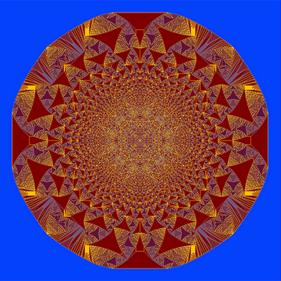
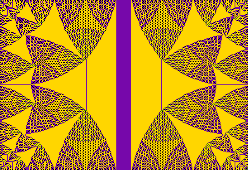
The Abelian sandpile model (ASM) was first introduced by Bak, Tang, and Wiesenfeld (1987). It is the foundational model of self-organized criticality, and is significant because complexity in the system emerged spontaneously, and it is therefore representative of natural systems without artificial constraints. Later, Dhar (1998) discovered that the model is considered abelian because the order of perturbations does not affect its final state.
Dynamics
Dynamics
The ASM, in a 2-dimensional representation, consists of the standard square lattice ℤ² with dimensions N x M. The starting configuration of the ASM assigns values to each site as represented as z₀(x,y). In addition, a common threshold value h is chosen and assigned to the system; for example, a generic threshold of h=4, z₀ = {{0, 1}, {2, 3}}. From there, an individual grain of sand may be added to a site without changing the other vertices. If the site remains stable, the model can continue to iterate and add grains to other sites. If any one vertex passes the threshold, it is unstable, or zᵢ(xᵤ, yᵤ) >= 4 for (xᵤ, yᵤ) ∈ Γ. Symbolically, the height of the “sandpile” at the site has increased and the grains of sand topple. In the model, instability of a vertex leads leads it to collapse and spill grains onto adjacent sites, where
zᵢ(xᵤ, yᵤ) = zᵢ(xᵤ, yᵤ) -h and zᵢ(xᵤ ±1, yᵤ ±1) = zᵢ(xᵤ ±1, yᵤ ±1) + 1,
provided (xᵤ ±1, yᵤ ±1) ∈ Γ.
This, in turn, may lead to further avalanches that can extend throughout the entire lattice. If the vertex is located at a boundary (x = N or y = M), grains without an adjacent site exit the system.
zᵢ(xᵤ, yᵤ) = zᵢ(xᵤ, yᵤ) -h and zᵢ(xᵤ ±1, yᵤ ±1) = zᵢ(xᵤ ±1, yᵤ ±1) + 1,
provided (xᵤ ±1, yᵤ ±1) ∈ Γ.
This, in turn, may lead to further avalanches that can extend throughout the entire lattice. If the vertex is located at a boundary (x = N or y = M), grains without an adjacent site exit the system.
Abelian Sandpile Model
Abelian Sandpile Model
The first step in our project was to develop the Abelian Sandpile Model in Wolfram. We initially created our Abelian Sandpile Model to run on randomly generated grids while still being compatible with the EEG data when we combined the two.
First, we developed a function that topples a specific pile by moving grains of sand of that pile to neighboring piles when the original pile reaches a set threshold. The function takes the grid, the specific pile’s coordinates, and the dimensions of the grid, and outputs the grid after the specified pile has toppled. The threshold function first checks if the sandpile at the given coordinate is greater than the tipping point, and therefore needs to be toppled. If this is evaluated to be true, then it spreads the grains of sand onto adjacent sandpiles. In this case, the tipping point of the grid is 4.
Initial threshold function:
In[]:=
tippingPoint=4;threshold[grid_List,{x_Integer,y_Integer},dimension_Integer]:=Module[{localGrid},localGrid=grid;If[localGrid[[x,y]]>=tippingPoint,localGrid[[x,y]]-=tippingPoint;If[x<dimension,localGrid[[x+1,y]]++];If[x>1,localGrid[[x-1,y]]++];If[y>1,localGrid[[x,y-1]]++];If[y<dimension,localGrid[[x,y+1]]++]];localGrid]
Here is an example grid before it is toppled. The light purple color of the sandpile represents four grains.
In[]:=
exampleGrid={{0,0,0,0},{0,0,0,0},{0,0,4,0},{0,0,0,0}};ArrayPlot[exampleGrid,ColorRules->{0->White,1->Yellow,2->LightOrange,3->LightRed,4->LightMagenta}]
Out[]=

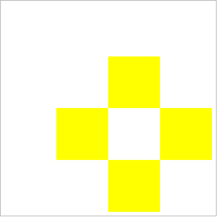
The pile is unstable because it is over the tipping point, so it topples and its grains are moved to nearby sandpiles.
The four yellow sandpiles each represent one grain, and they add up to the four grains that were originally in the light purple sandpile before it was toppled.
In[]:=
ArrayPlot[threshold[exampleGrid,{3,3},4],ColorRules->{0->White,1->Yellow,2->LightOrange,3->LightRed,4->LightMagenta}]
Out[]=
Next, to topple entire grids instead of just one sandpile, we expanded this function to successively topple one pile after another until the whole grid was toppled.
In[]:=
oneTopple[grid_List]:= Last[FoldList[threshold[#1,#2,Length[grid]]&,grid, Partition[Riffle[Flatten[ConstantArray[#,Length[grid]]&/@Range[Length[grid]]],Flatten[ConstantArray[Range[Length[grid]],Length[grid]]]],2]]]
However, toppling the entire grid does not ensure that the entire grid had stabilized, as a topple of one sandpile can make another sandpile critical again. Thus, we needed to continuously apply this function to the grid until the entire grid was stabilized.
To do this, we created another function that would check if there were any sandpiles in the grid that were still critical, and it returns True or False.
In[]:=
checkCritical[grid_List]:= Module[{critical},critical = AnyTrue[Flatten[grid], # >= 4 &]; critical]
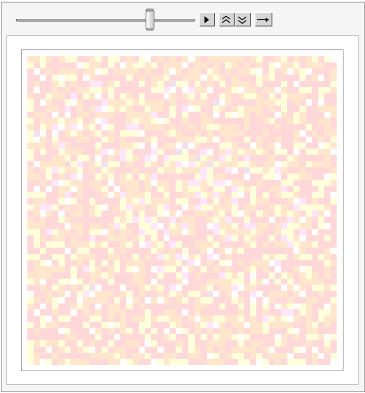
Combining this function with the function that topples the entire grid, we were able to continuously topple any grid until it was completely stabilized. We also wanted to be able to represent this data in an animation and keep track of the different avalanches during the stabilization, instead of just recording the starting and ending grids, so we used ArrayPlot on all topples of the grid. We also assigned different colors to different values of grains in sandpiles to better visualize the data. Generally, as the colors get darker, the number of grains in the sandpile increases. In this case, all colors that are darker than light purple are unstable.
This function iterates until a period of stability is reached.
In[]:=
allTopples[grid_List]:= NestWhileList[oneTopple,grid,checkCritical]
This function animates the list of grids using ListAnimate:
In[]:=
sandpileAnimate[grid_List]:= ListAnimate[Map[ArrayPlot[#, ColorRules->{0->White,1->LightYellow,2->LightOrange,3->LightRed, 4->LightMagenta, 5->LightPurple,6->Yellow,7->Orange,8->Red,9->Magenta,10->Purple,11->Darker[Orange],12->Darker[Red],13->Darker[Magenta],14->Darker[Purple]}]&, allTopples[grid]], AnimationRunning->False]
Here is an example animation of a randomly generated 50x50 grid stabilizing.
In[]:=
AnimatedImage[Import[CloudObject["https://www.wolframcloud.com/obj/c5690f9b-52ed-4185-9080-a02a0d252bac"],"GIF"],ImageSize->Medium]
Out[]=
As another example, if the entire grid is just below the threshold, and you run it through the toppling function, nothing would happen
Combining the ASM and EEG
Combining the ASM and EEG
Dataset
Dataset
Here are our imported datasets from an MDPI article called “Electroencephalograms during Mental Arithmetic Task Performance.” These datasets contain electroencephalography data, which measures brain activity by recording electrical signals at various sections of the scalp. These recordings were taken from 36 subjects every 0.3 seconds while performing mental arithmetic. Each of the csv files below represents one person. The complete datasets contain over 30 thousand recordings from each of the 36 people, so we took every 100th line of recordings for a smaller but evenly distributed sample of the data. Thus, each row of the dataset below (which is one out of the five that we’re using) represents the EEG recordings of the brain every 30 seconds, and each number in the row represents the specific amount of activity at the corresponding electrode placement according to the International 10/20 electrode placement system, which results in 19 electrodes at channels Fp1, Fp2, F3, F4, F7, F8, T3,T4, C3, C4, T5, T6, P3, P4, O1, O2, Fz, Cz, and Pz.
This is the 10-20 system of EEG electrode placement that our dataset uses
This function creates a list of the electrical activity associated with each electrode.
For example, here is row 100 of the first dataset with each electrode with its corresponding electrical activity:
Then, this function takes the list from the previous function and turns it into a 5x5 square lattice that follows the 10-20 EEG electrode placement.
This is the starting plot of row 100:
We can then run this output through our Abelian Sandpile model:
We then created grids of all data in the first EEG dataset, and ran each row through the Abelian Sandpile Model we developed.
Here are some sample animations of simulated neuronal avalanches:
Power-Law Distribution Analysis
Power-Law Distribution Analysis
We created a function to detect topples, which occurs when the value of a cell decreases.
We then wrote a function for tracking avalanche sizes throughout a full Abelian Sandpile Model simulation.
This function uses the detectTopples function to locate topples and track avalanche sizes by tracing each topple.
We mapped the track Avalanches function on the first EEG dataset to detect the different avalanche sizes during each simulation.
We then reformatted the avalanche sizes into a list with each avalanche size and amount:
Next, we took the logarithm of each list, and deleted any cases with log0 since this is undefined.
We then took the data and separated it into x and y components to graph.
This is a log-log plot of the data in the first EEG dataset.
We also created linear model of the data.
The first EEG dataset has a strong linear correlation, indicating a power-law distribution.
This code simply graphs the linear regression of the plot with the data.
The model’s R-squared, or the measure of how well the regression model explains the variability of the dependent variable, ranging from 0 (no fit) to 1 (perfect fit):
The model’s R, which is the correlation coefficient, measuring the strength and direction of the linear relationship between the two variables.
We then created a function that streamlines the previous steps, combining them into one function. The dataset being plotted is inputted, and it outputs the graph, linear regression, and R value.
Here is the first EEG dataset’s model, as displayed above.
This is the second EEG dataset’s model. This has the lowest linear correlation, but it is still relatively linear.
This is the third EEG dataset’s model.
This is the fourth EEG dataset’s model.
This is the fifth EEG dataset’s model.
Through analyzing our simulations, we determined strong linear correlations (0.79+) between the size and frequency of recorded avalanches. Since these avalanches represent neuronal avalanches, the results indicate a power-law distribution, providing evidence for the critical brain hypothesis.
Conclusion
Conclusion
This study implements the Abelian Sandpile model using the Wolfram Language and also applies it to selected electroencephalogram (EEG) data to explore the dynamics of neuronal activity. The analysis of the simulations from the abelian sandpile model show a power-law distribution, supporting the hypothesis of self-organized criticality in the brain. These findings emphasize the potential of models (such as the abelian sandpile model) to demonstrate the connection between neuronal avalanches and critical states in the brain. In this work, we extend the application of this foundational model to what is widely considered the most intricate system in existence: the human brain. By utilizing EEG data from 19 electrodes in the 10/20 system, we simulated neuronal avalanches and analyzed their power-law distribution, bridging theoretical modeling with experimental data. The observed evidence of a power-law distribution not only substantiates the critical brain hypothesis of neuroscience but also offers a novel computational lens through which to study self-organized criticality in neuronal systems.
Future Work
Future Work
In the future, we would also like to compare the result of our simulations of brain activity to the actual data to show how the ASM is a good representation of how the brain operates. Using our simulated data and real data, we could compare the two and find areas of similarity and of error. Additionally, given more time, we would use data from more subjects not only this experiment but from others too, to have more samples of data and evidence for the critical brain hypothesis. We would like to compare the simulated avalanches against real avalanches to determine model accuracy. We are also interested in exploring 3-dimensional mapping and adjusting model parameters to better simulate electrode relations in the brain. We would also like to calculate entropy to determine complexity.
Acknowledgements
Acknowledgements
We would like to thank George Woodrow, our mentor, for his support and helpfulness during this project. We would also like to thank Eryn Gillam and Rory Foulger for organizing WELP.
References
References
◼
Abelian sandpile model. (2023, May 9). Wikipedia. https://en.wikipedia.org/wiki/Abelian_sandpile_model
◼
Anand, A. (2020). Complete EEG dataset. Kaggle.com. https://www.kaggle.com/datasets/amananandrai/complete-eeg-dataset?resource=download&select=s00.csv
◼
A Physical Theory For When the Brain Performs Best | Quanta Magazine. (2023, January 31). Quanta Magazine. https://www.quantamagazine.org/a-physical-theory-for-when-the-brain-performs-best-20230131/
◼
Dhar, D. (1998). The Abelian sandpile and related models. 263(1-4), 4–25. https://doi.org/10.1016/s0378-4371(98)00493-2
◼
Lang, M., & Shkolnikov, M. (2019). Harmonic dynamics of the abelian sandpile. Proceedings of the National Academy of Sciences, 116(8), 2821–2830. https://doi.org/10.1073/pnas.1812015116
◼
Marković, D., & Gros, C. (2014). Power laws and self-organized criticality in theory and nature. Physics Reports, 536(2), 41–74. https://doi.org/10.1016/j.physrep.2013.11.002
◼
Zyma, I., Tukaev, S., Seleznov, I., Kiyono, K., Popov, A., Chernykh, M., & Shpenkov, O. (2019). Electroencephalograms during Mental Arithmetic Task Performance. Data, 4(1), 14. https://doi.org/10.3390/data4010014
CITE THIS NOTEBOOK
CITE THIS NOTEBOOK
Exploring brain criticality with the Abelian sandpile model
by Wolfram Education Programs
Wolfram Community, STAFF PICKS, February 4, 2025
https://community.wolfram.com/groups/-/m/t/3379955
by Wolfram Education Programs
Wolfram Community, STAFF PICKS, February 4, 2025
https://community.wolfram.com/groups/-/m/t/3379955