ABSTRACT (original article): The present paper describes how to apply the Chebyshev orthogonal collocation technique to solve steady-state and unsteady-steady two-dimensional problems. All problems are solved using one single computer algebra, Mathematica©. The problems include: (1) steady-state heat transfer in a rectangular bar, (2) steady-state flow in a rectangular duct, (2) steady-state heat transfer in a cooling cylindrical pin fin, (4) steady-state heat conduction in an annulus, (5) unsteady-state heat transfer in a rectangular bar, and finally (6) unsteady-state diffusion reaction system. Whenever possible the results obtained with orthogonal collocation are compared to the analytical solution in order to validate the applied numerical technique. CITATION (original article): Binous, H., Kaddeche, S., & Bellagi, A. (2015). Solving two-dimensional chemical engineering problems using the chebyshev orthogonal collocation technique. In Computer Applications in Engineering Education (Vol. 24, Issue 1, pp. 144–155). Wiley. DOI: https://doi.org/10.1002/cae.21680
In electronic systems, a fin is a heat sink or a passive heat exchanger that cools a device by dissipating heat into the surrounding medium (e.g. air). This diagram shows a cylindrical pin fin, used to maximize heat transfer to a fluid between two walls:
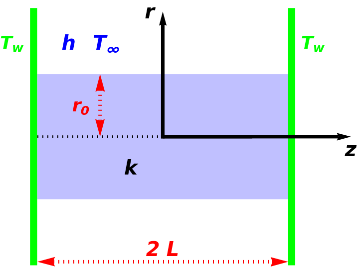
The walls are at a high temperature . The fluid flowing over the pin has a free stream temperature . The heat transfer coefficient between the pin wall and the surrounding medium is labeled (in ). If one introduces the dimensionless temperature , the governing equation is:r +ϕ=0,with and .
T
w
T
∞
h
W/K
2
m
ϕ=-
T-
T
∞
T
w
T
∞
1
r
∂
∂r
∂ϕ
∂r
2
∂
∂
2
z
0≤r≤
r
0
0≤z≤L
The associated boundary conditions are then:=0 (axial symmetry condition),=0 (radial symmetry condition),+ϕ=0 (continuity of heat flux at the boundary fin/surrounding air), and (constant temperature at the wall),where is the thermal conductivity of the cylindrical pin fin and =1.
∂ϕ
∂z
z=0
∂ϕ
∂r
r=0
∂ϕ
∂r
h
k
r=
r
0
ϕ(z=L)==1
ϕ
w
k (W/m K)
r
0
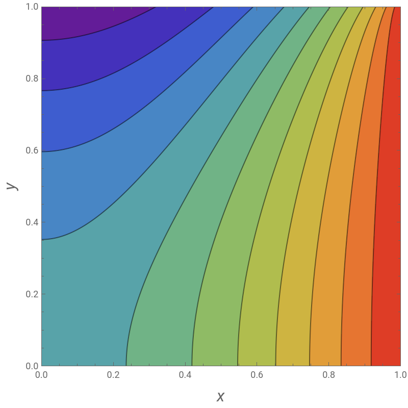
We plot the contours of the dimensionless temperature for a Biot number, Bi=1. This solution is based on Chebyshev orthogonal collocation with collocation points. The analytical solution of the differential equation obtained by separation of variables [2] is given by:,where = is the Biot number and are the zeros of the nonlinear function: . These roots are reported in Table 3 of Ref. 2 and could be obtained using Wagon’s graphical method (see Ref. 3).We find good agreement between our numerical solution and the analytical solution plotted in Ref. 2. Finally, we find excellent agreement between contour plots obtained using Mathematica and Python.
N=41
ϕ=
∞
∑
n=1
2 ( r)cosh( z)
B
i
J
0
λ
n
λ
n
cosh( L)()+
λ
n
J
0
λ
n
r
0
2
()
λ
n
r
0
2
B
i
B
i
h
r
0
k
λ
n
f(λ)=(λ )(λ )-(λ )
r
0
J
1
r
0
J
0
r
0
B
i
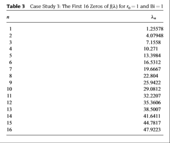
Parameters of the problem reproduced from Ref . 2.
In[]:=
r0=1;Bi=1(*Biotnumber*);
Numerical solution based on Orthogonal Collocation and the Gauss - Lobatto nodes
Derivative Matrices constructed using 41 Gauss - Lobatto collocation points
In[]:=
Np=40;Ds=Table[d[i,j],{i,0,Np},{j,0,Np}];d[0,0]=(2Np^2+1)/6//N;d[Np,Np]=-(2Np^2+1)/6//N;d[i_,i_]:=-y[i]/(2(1-y[i]^2));y[i_]:=Cos[iPi/Np]//N;d[j_,k_]:=If[j≠k,c[j](-1)^(j+k)/(c[k](y[j]-y[k]))];c[i_]:=If[i0||iNp,2,1];Dsq=Ds.Ds;
In[]:=
L2a=4KroneckerProduct[Dsq,IdentityMatrix[Np+1]];L2b=4KroneckerProduct[IdentityMatrix[Np+1],Dsq];Lbc1=2KroneckerProduct[IdentityMatrix[Np+1],Ds];Lbc2=2KroneckerProduct[Ds,IdentityMatrix[Np+1]];
Governing equations
In[]:=
x=Table[r0/2(1+y[i]),{i,Np,0,-1}];
In[]:=
U=Table[u[i+(j-1)(Np+1)],{j,1,Np+1},{i,1,Np+1}]//Flatten;
In[]:=
Eq[i_]:=L2a[[i]].U+L2b[[i]].U-1/x[[Quotient[i-1,Np+1]+1]]Lbc2[[i]].U0;
In[]:=
bc1=Table[Lbc1[[1+(j-1)(Np+1)]].U0,{j,1,Np+1}];bc2=Table[Lbc2[[i+Np(Np+1)]].UBi/r0u[i+Np(Np+1)],{i,2,Np}];bc3=Table[Lbc2[[i]].U0,{i,2,Np}];
In[]:=
sys=Join[{bc1,bc2,bc3,Table[u[Np+1+(j-1)(Np+1)]1,{j,1,Np+1}],Table[Eq[i+(j-1)(Np+1)],{j,2,Np},{i,2,Np}]}]//Flatten;
In[]:=
initguess=Flatten[Table[{u[i+(j-1)(Np+1)],0.5},{j,1,Np+1},{i,1,Np+1}],1];
Solution using FindRoot
In[]:=
sol=Quiet@FindRoot[sys,initguess];
Contour plot of the solution
In[]:=
a=Flatten[Table[{x[[i]],x[[j]],u[i+(j-1)(Np+1)]/.sol},{j,1,Np+1},{i,1,Np+1}],1];f=Interpolation[a,InterpolationOrder3];
In[]:=
p1=ContourPlot[f[x1,y1],{x1,0,r0},{y1,0,r0},ContoursTable[0.05i,{i,1,20,1}],PlotPoints100,ImageSize{400,400},FrameLabel{Style["x",Italic,16],Style["y",Italic,16]},PlotLegendsAutomatic,ColorFunction"Rainbow",PlotRange->{{0,1},{0,1}}]
Out[]=

In[]:=
p1=ContourPlot[f[x1,y1],{x1,0,r0},{y1,0,r0},ContoursTable[0.05i,{i,1,20,1}],PlotPoints100,ImageSize{400,400},FrameLabel{Style["x",Italic,16],Style["y",Italic,16]},PlotLegendsAutomatic,ContourStyle->Table[{Dashed,Darker@Red,Thick},{i,1,20,1}],ContourShading->None,PlotRange->{{0,1},{0,1}}]
Out[]=
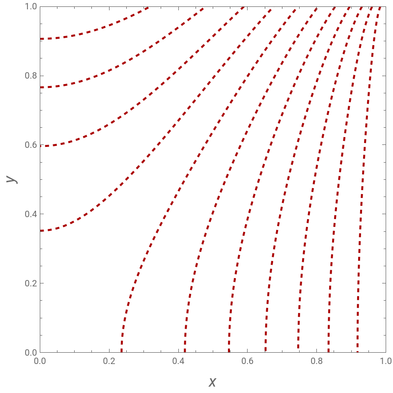
Bennett' s solution + our numerical solutions superimposed on the same plot
References
References
◼
[1] H. Binous, S. Kaddeche and A. Bellagi, Solving two-dimensional chemical engineering problems using the chebyshev orthogonal collocation technique, Computer Applications in Engineering Education, 24(1), pp. 144-155, 2016. https://onlinelibrary.wiley.com/doi/abs/10.1002/cae.21680
◼
[2] T. Bennett, Transport by Advection and Diffusion, New York: Wiley, 2012.
◼
[3] S. Wagon, Mathematica in action: Problem solving through visualization and computation, 3rd ed. Springer-Verlag, Berlin, 2010.
CITE THIS NOTEBOOK
CITE THIS NOTEBOOK
Cooling by a cylindrical pin fin
by Housam Binous and Ahmed Bellagi
Wolfram Community, STAFF PICKS, March 24, 2024
https://community.wolfram.com/groups/-/m/t/3146557
by Housam Binous and Ahmed Bellagi
Wolfram Community, STAFF PICKS, March 24, 2024
https://community.wolfram.com/groups/-/m/t/3146557