Wolfram Cloud Document

ABSTRACT (original article): In this work, we study spherically symmetric vacuum solutions in one-parameter new general relativity (NGR), a specific theory in teleparallel gravity which is constructed from the three possible quadratic scalars obtained from torsion with arbitrary coefficients satisfying the requirements for the absence of ghosts. In this class of modified theories of gravity, the observable effects of gravity result from the torsion rather than the curvature of the spacetime. Unlike in GR, where the fundamental quantity is the metric from which the Levi-Civita connection is derived, in teleparallel theories of gravity the fundamental variable is the tetrad, from which one constructs the metric and the teleparallel connection. We consider the most general tetrad for spherical symmetry and we derive the corresponding field equations. Under adequate assumptions, we find three different branches of vacuum solutions and discuss their associated phenomenology. In particular, we analyze the photon sphere, the classical tests of GR such as the light deflection, the Shapiro delay, and the perihelion shift, and also the Komar mass, while providing a detailed comparison with their Schwarzschild spacetime counterparts. Finally, we analyze how the observational imprints from accretion disks and shadows are affected in comparison with their GR counterparts, and conclude that the free parameters of the model might induce additional attractive or repulsive effects to the propagation of photons, depending on their values. CITATION (original article): Rosa, João Luís and Cordeiro, Daniela S. J. and Macedo, Caio F. B. and Lobo, Francisco S. N. (2024), Observational imprints of gravastars from accretion disks and hot spots. Phys. Rev. D 109, 084002. https://doi.org/10.1103/PhysRevD.109.084002. Code Coauthors: Gonzalo Olmo and Diego Rubiera-Garcia

Faster integration algorithm

Detailed algorithm available at the end of this notebook

Definitions

In this section, we define the necessary quantities and functions to produce the observables that follow.

In[]:=

Needs["PlotLegends`"]//QuietSetDirectory[NotebookDirectory[]];

General definitions

Geometrical quantities

Number of dimensions and system of coordinates. By default, we work in 4 dimensions and we consider a system of spherical coordinates.

ND=4;X={t,r,θ,ϕ};

Metric tensor describing the spacetime. In general, the spacetime can be decomposed into an interior and an exterior regions. Usually, the exterior region is vacuum, thus corresponding to the Schwarzschild spacetime. The interior region can vary depending on the spacetime under analysis. For the purpose of this notebook, we consider the interior spacetime to be that of a thin-shell gravastar of mass M and radius R. This thin-shell gravastar has a constant density

. The additional free parameter of the model α, controls the mass distribution of the gravastar, varying from a maximum value α=1 corresponding to a star with the entire mass distributed in its volume, to

α=

min

, where

min

depends on the model, for which the mass is entirely distributed on the surface of the star.

ge=DiagonalMatrix[{gtte,grre,gθθe,gϕϕe}];gtte=-(1-(2M)/r);grre=

-1

(1-(2M)/r)

;gθθe=

;gϕϕe=

Sin[θ]

;gi=DiagonalMatrix[{gtti,grri,gθθi,gϕϕi}];gtti=-α(1-(2m[r])/r);grri=

-1

(1-(2m[r])/r)

;gθθi=

;gϕϕi=

Sin[θ]

;m[r_]:=(4/3)ρ0Pi

ρ0=(3Mρ)(4π

);Mρ=(2M+R(-1+α))/(2α);

To compute the geometrical quantities of interest in this spacetime, we need the inverse metric, the determinant of the metric, and the square-root of the absolute value of the metric determinant. These are calculated separately for the interior and the exterior metrics. The geometrical quantities of interest are the Christoffel symbols, the Riemann tensor, the Ricci tensor, the Ricci scalar, and the Einstein’s tensor. Although these quantities are not used explicitly in this notebook, they are useful for other analyses that the reader might be interested in, and thus we provide them explicitly.

Ae=Inverse[ge];(*inversadamétrica*)he=FullSimplify[Det[ge]];(*determinantedamétrica*)Ge=Sqrt[-he];(*raizdodeterminante*)Ai=Inverse[gi];(*inversadamétrica*)hi=FullSimplify[Det[gi]];(*determinantedamétrica*)Gi=Sqrt[-hi];(*raizdodeterminante*)

Christoffel symbols

Γe=Simplify[Table[Sum[(1/2)*Ae[[a,d]]*(D[ge[[d,c]],X[[b]]]+D[ge[[d,b]],X[[c]]]-D[ge[[b,c]],X[[d]]]),{d,1,ND}],{a,1,ND},{b,1,ND},{c,1,ND}]];Γi=Simplify[Table[Sum[(1/2)*Ai[[a,d]]*(D[gi[[d,c]],X[[b]]]+D[gi[[d,b]],X[[c]]]-D[gi[[b,c]],X[[d]]]),{d,1,ND}],{a,1,ND},{b,1,ND},{c,1,ND}]];

Riemann tensor

Rabcde=Simplify[Table[Sum[ge[[f,h]](D[Γe[[f,b,d]],X[[c]]]-D[Γe[[f,b,c]],X[[d]]]+Sum[Γe[[e,b,d]]*Γe[[f,e,c]]-Γe[[e,b,c]]*Γe[[f,e,d]],{e,1,ND}]),{f,1,ND}],{h,1,ND},{b,1,ND},{c,1,ND},{d,1,ND}]];Rabcdi=Simplify[Table[Sum[gi[[f,h]](D[Γi[[f,b,d]],X[[c]]]-D[Γi[[f,b,c]],X[[d]]]+Sum[Γi[[e,b,d]]*Γi[[f,e,c]]-Γi[[e,b,c]]*Γi[[f,e,d]],{e,1,ND}]),{f,1,ND}],{h,1,ND},{b,1,ND},{c,1,ND},{d,1,ND}]];

Ricci tensor

Rabe=Simplify[Table[Sum[Ae[[c,d]]*Rabcde[[d,a,c,b]],{c,1,ND},{d,1,ND}],{a,1,ND},{b,1,ND}]];Rabi=Simplify[Table[Sum[Ai[[c,d]]*Rabcdi[[d,a,c,b]],{c,1,ND},{d,1,ND}],{a,1,ND},{b,1,ND}]];

Ricci scalar

Rse=Simplify[Sum[Ae[[a,b]]*Rabe[[a,b]],{a,1,ND},{b,1,ND}]];Rsi=Simplify[Sum[Ai[[a,b]]*Rabi[[a,b]],{a,1,ND},{b,1,ND}]];

Einstein’s tensor

Gabe=SimplifyTableRabe[[a,b]]-

Rsege[[a,b]],{a,1,ND},{b,1,ND};Gabi=SimplifyTableRabi[[a,b]]-

Rsigi[[a,b]],{a,1,ND},{b,1,ND};

For any non-vacuum spacetime like the ones describing alternatives to the black-hole hypothesis, one also needs to define an appropriate stress-energy tensor describing the matter fields. For the purpose of this work, we consider a stress-energy tensor that is diagonal, i.e., no heat-fluxes or shear are present, and that is isotropic, i.e., the pressure components are the same in every direction. We provide the stress-energy tensor written as a mixed tensor, and then compute the totally covariant and contravariant tensors. Again, these are not used explicitly in this notebook, but might be useful for the reader in other contexts.

Tmis=DiagonalMatrix[{-ρ[r],p[r],p[r],p[r]}];Tem=Table[Sum[gi[[c,b]]Tmis[[a,c]],{c,1,ND}],{a,1,ND},{b,1,ND}];Tin=Table[Sum[Ai[[a,c]]Tmis[[b,c]],{c,1,ND}],{a,1,ND},{b,1,ND}];

Finally, we provide the definitions of the covariant derivatives for scalar functions, first-order, and second-order tensorial quantities with covariant, contravariant, and mixed indices. These are useful e.g. to compute the field equations or the equations of motion of any additional fields, in case the reader is interested.

CovDs[S_]:=Table[D[S,X[[a]]],{a,1,ND}]CovDd[V_]:=Table[D[V[[b]],X[[a]]]-Sum[Γ[[c,a,b]]V[[c]],{c,1,ND}],{a,1,ND},{b,1,ND}]CovDu[V_]:=Table[D[V[[b]],X[[a]]]+Sum[Γ[[b,a,c]]V[[c]],{c,1,ND}],{a,1,ND},{b,1,ND}]CovDdd[V_]:=Table[D[V[[b,c]],X[[a]]]-Sum[Γ[[d,a,b]]V[[d,c]],{d,1,ND}]-Sum[Γ[[d,a,c]]V[[b,d]],{d,1,ND}],{a,1,ND},{b,1,ND},{c,1,ND}]CovDuu[V_]:=Table[D[V[[b,c]],X[[a]]]+Sum[Γ[[b,a,d]]V[[d,c]],{d,1,ND}]+Sum[Γ[[c,a,d]]V[[b,d]],{d,1,ND}],{a,1,ND},{b,1,ND},{c,1,ND}]CovDud[V_]:=Table[D[V[[b,c]],X[[a]]]-Sum[Γ[[d,a,c]]V[[b,d]],{d,1,ND}]+Sum[Γ[[b,a,d]]V[[d,c]],{d,1,ND}],{a,1,ND},{b,1,ND},{c,1,ND}]

Accretion disk models

The intensity profiles of the accretion disks in the reference frame of the emitter are described by a Johnson’s-SU distribution. Depending on the type of accretion disk we are interested in, the values of the free parameters of the disk can be modified. For example, one may be interested in accretion disks that are truncated at the radius of the Innermost Stable Circular Orbit (ISCO), or at the radius of the Lighr-ring (LR), etc. In this work, we use two types of accretion disks: the one truncated at the radius of the ISCO, given that the orbits of particles become unstable at radii smaller than that, and a second one denoted by C model that extends all the way down to the center of the gravastar, with the objective of verifying how a potential accumulation of matter in the interior could affect the observational properties of the spacetime.

In[]:=

Int[r_,γ_,μ_,σ_]:=

Exp-

γ+ArcSinh

r-μ





(r-μ)

IntISCO[x_]:=Intr,-2,6,

IntLR[x_]:=Intr,-2,3,

IntEH[x_]:=Intr,-3,2,

IntC[x_]:=Int[r,0,0,2]Plot[{IntISCO[r],IntLR[r],IntC[r],IntEH[r]},{r,0,11},PlotRangeAll,PlotRangeAll,PlotStyle{Red,{Blue,Dashed},{Purple,Dotted},{Orange,DotDashed}},FrameTrue,BaseStyle14,FrameLabel{"r / M","I(r)"},PlotLegend{"ISCO","LR","Centre","EH"},LegendShadowNone,LegendSize{0.35,0.35},LegendPosition{0.45,0.2}]Plot[{IntISCO[r],IntC[r]},{r,0,11},PlotRangeAll,BaseStyle12,FrameStyleBlack,PlotTheme"Scientific",PlotStyle{Red,{Blue,Dashed}},FrameTrue,BaseStyle14,FrameLabel{"r / M","M

(r)"},PlotLegend{"ISCO","Centre"},LegendShadowNone,LegendSize{0.35,0.3},LegendPosition{0.45,0.2}]

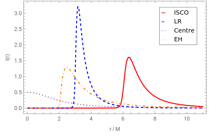
Out[]=

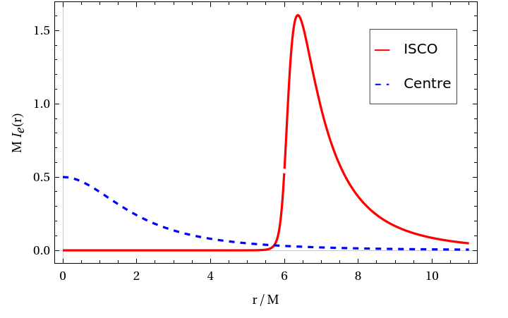
Composed metric

In case the metric describing the spaccetime has an interior and an exterior component, like it happens for the gravastar models analyzed in this work, it is necessary to connect the two metrics into a single metric function. In this section, we produce the composed metric function and provide plots to show how the metric varies with respect to the two independent parameters of the model, namely the radius R and the parameter α controlling the mass distribution.

Functions for axial ray - tracing

Geodesic Integrator

This function integrates the geodesic equation and produces the trajectory of a single photon. The parameters of the function are: the radius of the observer, the initial impact parameter, the observational angle (in this section it vanishes by default given that we are interested in axial observations), and the two free parameters of the star. The trajectories are saved in the quantities Sol0 and Sol1 for later use.

Integration Loop

This function takes a range of impact parameters from b0i to bend, and a number of steps Nstep, and runs the geodesic integrator function from the previous section for several geodesics inside the range provided. Depending on the number of times the geodesic crosses the equatorial plane, the function saves the impact parameter and the radius at which that intersection happens in different lists ListRi for later use. The Second function does precisely the same as the first one but only for a range of impact parameters close to the critical impact parameter, in order to produce additional data in the region where geodesics are the most unstable.

Shadow Producer

This function takes the same arguments as the previous functions, plus the accretion disk model, and the names of three files on which to write the data for the observed indensity profiles, shadow images, and the image itself. The function starts by calling the geodesic loop to produce a congruence of geodesics, and extract the values of the radius for which the geodesics intersect the equatorial plane. Then, the function takes the value of the intensity of the accretion disk model at this radius and calculates the observed intensity in the reference frame of the observer through the analysis of the gravitational redshift. Finally, the function plots the observed image on the reference frame of the observer. The two functions given do the same calculation but through two slightly different methods.

Functions for inclined ray - tracing

Geodesic Integrator

Similarly to the axial case, this function integrates the geodesic equation. However, an additional parameter is given, the number of angle steps Nangles, between 0 and π. For each of these angles, the function takes an inclined plane and computes the intersections between the geodesic and the equatorial plane as seen from that particular inclined angle.

Integration Loop

This function loops through an interval of impact parameters and produces the geodesic congruences in that interval. Again, there is one additional parameter in comparison with the axial case, that is the number of angle steps.

Shadow Producer

Finally, this function follows the same procedure as in the axial case to produce the observed intensity profiles in the reference frame of the observer. The difference stands on the fact that the intensity profile varies depending on the observation angle, and thus the observed image is no longer circularly symmetric.

Testing the functions

In this section, we test the numerical functions defined in the previous section.

Geodesic Integrator

We can test the geodesic integrator function for a given input and produce the corresponding geodesic.

Geodesic Loop

We can also do the same for a congruence of N geodesics.

Shadow Producer

We can produce the observed image of our model as seen from the vertical axis for different metrics and accretion disk models

Inclined Shadow Producer

And the same can be done also for inclined observations

Produce Images

Intensity Plots

And we produce the observed intensity profiles for the models considered

Detailed algorithm

Density profiles

SU MODELS

We set the fudge factor

SU1

We start with the algorithm to produce images

The final image is found

SU2

SU10

Other publications that use this code

◼

“Spherically symmetric vacuum solutions in 1-Parameter New General Relativity and their phenomenology”, H. Asuküla, S. Bahamonde, M. Hohmann, V. Karanasou, C. Pfeifer and J. L. Rosa, [arXiv:2311.17999 [gr-qc]].

◼

“The optical appearance of a nonsingular de Sitter core black hole geometry under several thin disk emissions”; I. De Martino, R. Della Monica, and D. Rubiera-Garcia; Phys. Rev. D, in press arXiv:2310.11039 [gr-qc].

◼

“Photon rings as tests for alternative spherically symmetric geometries with thin accretion disks”, L. F. Dias da Silva, F. S. N. Lobo, G. J. Olmo, and D. Rubiera-Garcia , Phys. Rev. D 108 (2023) 8, 084055 [arXiv: 2307.06778 [gr-qc]].

◼

“Observational properties of relativistic fluid spheres with thin accretion disks”, J. L. Rosa, Phys. Rev. D107, no.8, 084048 (2023), [arXiv:2302.11915 [gr-qc]].

◼

“Shadows and photon rings of regular black holes and geonic horizonless compact objects”, G. J. Olmo, J. L. Rosa, D. Rubiera-Garcia and D. Sáez-Chillón Gómez , Class. Quant. Grav, 40 (2023) 17, 174002 [arXiv:2302.12064 [gr-qc]].

◼

“Imaging compact boson stars with hot-spots and thin accretion disks”, J. L. Rosa (first author), C. Macedo, and D. Rubiera-Garcia, Phys. Rev. D, 108 (2023) 4, 044021 [arXiv:2303.17296 [gr-qc]].

◼

“Shadows of boson and Proca stars with thin accretion disks”; J. L. Rosa, D. Rubiera-Garcia; Phys. Rev. D 106 (2022) 8, 084004 [arXiv:2204.12949 [gr-qc]].

◼

“Multi-ring images of thin accretion disk of a regular naked compact object”; M. Guerrero, G. J. Olmo, D. Rubiera-Garcia, D. Sáez-Chillón Gómez ; Phys. Rev. D 106 (2022) 4, 044070 [arXiv:2205.12147 [gr-qc]].

◼

“Light ring images of double photon spheres in black hole and wormhole space-times”; M. Guerrero, G. J. Olmo, D. Rubiera-Garcia, D. Sáez-Chillón Gómez; Phys. Rev. D 105 (2022) 8, 084057 [arXiv:2202.03809 [gr-qc]].

◼

“New light rings from multiple critical curves as observational signatures of black hole mimickers”; G. J. Olmo, D. Rubiera-Garcia; D. Sáez-Chillón Gómez , Phys. Lett. B 829 (2022) 137045 [arXiv:2110.10002 [gr-qc]].

◼

“Shadows and optical appearance of black bounces illuminated by a thin accretion disk”; M. Guerrero, G. J. Olmo, D. Rubiera-Garcia, D. Sáez-Chillón Gómez , JCAP 08 (2021) 036 [arXiv:2105.15073 [gr-qc]].

CITE THIS NOTEBOOK

Observational imprints of gravastars from accretion disks and hot-spots
by João Luís Rosa, Daniela S. J. Cordeiro, Caio F. B. Macedo, Francisco S. N. Lobo, Gonzalo Olmo and Diego Rubiera-Garcia
Wolfram Community, STAFF PICKS, February 15, 2024
https://community.wolfram.com/groups/-/m/t/3123629