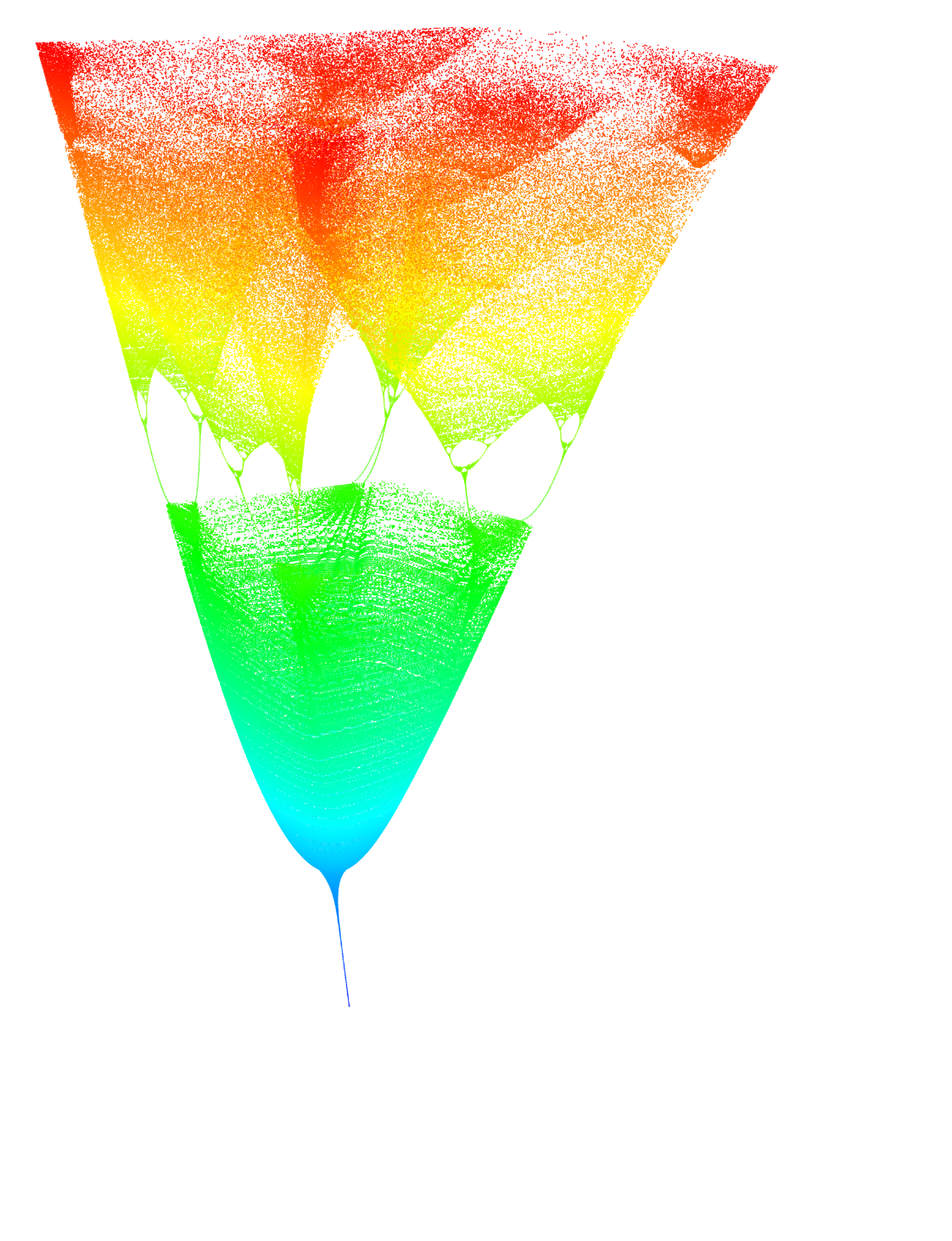
On the excellent blog of John D. Cook, there is a generalization of the logistic map bifurcation diagram for 3D: https://www.johndcook.com/blog/2021/07/31/3d-bifurcation-diagram/
I have attempted to reproduce it:
2D Bifurcation
2D Bifurcation
Logistic map for 2D
In[]:=
ClearAll[f];f[r_][{x_}]:={r[[1]]x(1-x)}
Create a 2D plot using the slice function defined in initialization section below.
In[]:=
ClearAll[bifurcation2d]bifurcation2d[f_,opts:OptionsPattern[{slice,"Step"->0.1}]]:=Graphics[{PointSize[0.001],Point[Flatten[Quiet@Table[slice[{r},f,FilterRules[{opts},Options[slice]]],{r,0.0,4.0,OptionValue["Step"]}],1]]},PlotRange{{0.,4.},{-0.2,1.0}},AxesTrue,AxesOrigin{0,-0.2}]
In[]:=
bifurcation2d[f,"Step"->0.006]
Out[]=
3D Bifurcation
3D Bifurcation
Logistic map for 3D
In[]:=
ClearAll[g];g[b_][{a_}][{x_,y_}]:={a-y(bx+(1.0-b)y),x+y*y/100.0};
Create a 3D plot
In[]:=
ClearAll[bifurcation3d,colorSlice]colorSlice[r_][l_]:={Hue[1.0-r/2.0,1,1],Point[l]};bifurcation3d[f_,opts:OptionsPattern[{slice,"Step"->0.1,"PointSize"->0.0015}]]:=Graphics3D[{PointSize[OptionValue["PointSize"]],Flatten[Quiet@Table[colorSlice[r]@slice[{r},f,FilterRules[{opts},Options[slice]]],{r,0.7,2.0,OptionValue["Step"]}],1]},AxesFalse,ViewVertical->{1.1,0.1,0},BoxRatios->{3,2,2},PlotRangeFull,BoxedFalse,ImageSizeFull]
In[]:=
g=bifurcation3d[g[0.25],"Step"->0.002,"Start"->{0.5,0.5},"Iteration"->1000]
Out[]=
Initializations
Initializations
Compute a slice of the bifurcation diagram for function f and parameter r. The function is attempting to detect a cycle to avoid having to always compute the maximum number of iterations.
In[]:=
ClearAll[slice];Options[slice]={"Drop"->100,"Iteration"->500,"Start"->{0.5}};slice[r_,f_,OptionsPattern[]]:=With[{roundFactor=10.0^5},Module[{res,x,z},res=<||>;x=Nest[f[r],OptionValue["Start"],OptionValue["Drop"]];Do[x=f[r][x];z=1.0*Round[x*roundFactor]/roundFactor;If[KeyExistsQ[res,z],Return[Flatten[Flatten[{r,#}]&/@Keys[res],1]],res[z]=True];,{n,OptionValue["Iteration"]}];Flatten[{r,#}]&/@Keys[res]]]