Phase Portrait of Lotka-Volterra Equation
Phase Portrait of Lotka-Volterra Equation


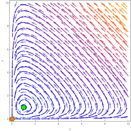
This Demonstration shows a phase portrait of the Lotka–Volterra equations, including the critical points. The eigenvalues at the critical points are also calculated, and the stability of the system with respect to the varying parameters is characterized.
Details
Details
The Lotka–Volterra equations are a pair of coupled differential equations
x
t
y
t
describing the dynamics of predator-prey populations, and , respectively.
y
x
References
References
[1] Wikipedia. "Lotka–Volterra Equations." (Jun 20, 2017) en.wikipedia.org/wiki/Lotka-Volterra_equations.
External Links
External Links
Permanent Citation
Permanent Citation
Wusu Ashiribo Senapon, Akanbi Moses Adebowale
"Phase Portrait of Lotka-Volterra Equation"
http://demonstrations.wolfram.com/PhasePortraitOfLotkaVolterraEquation/
Wolfram Demonstrations Project
Published: June 21, 2017