Consider the reversible reaction . This reaction involves three chemical species, , , and , and takes place in a packed bed reactor (PBR) with axial mixing. Our objective is to compare alternative solutions of this problem using Mathematica's NDSolve and using Chebyshev's orthogonal collocation method.
A+BC
k
f
⇌
k
r
A
B
C
Introduce the dimensionless parameters , = (Péclet number), and =kτ (Damköhler number). Then, the governing equations are:=-- r,=-- r,and =-+ r,where and =/.
τ=
L
u
P
e
uL
D
D
a
∂
C
A
∂t
1
P
e
2
∂
C
A
∂
2
x
∂
C
A
∂x
D
a
∂
C
B
∂t
1
P
e
2
∂
C
B
∂
2
x
∂
C
B
∂x
D
a
∂
C
C
∂t
1
P
e
2
∂
C
C
∂
2
x
∂
C
C
∂x
D
a
r=-
C
A
C
B
C
C
K
e
K
e
k
f
k
r
Initially, the reactor contains only species and such that (x,t=0)=0.6mol/l and (x,t=0)=0.4mol/l. The feed to the reactor is also composed of only and such that (x=,t)=0.6mol/l and (x=,t)=0.4mol/l.
A
B
C
A
C
B
A
B
C
A
-
0
C
B
-
0
Part 1 - validation of the solution based on Chebyshev orthogonal collocation
Part 1 - validation of the solution based on Chebyshev orthogonal collocation
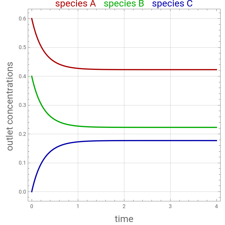
The code solves this system of partial differential equations for Péclet and Damköhler numbers equal to 5 and 3, respectively. The equilibrium constant is taken equal to 1. The Mathematica NDSolve results are shown as colored solid curves, while the Chebyshev orthogonal collocation values are shown as colored dots.
Clearly, the two approaches are in excellent agreement.
K
e
Clearly, the two approaches are in excellent agreement.
Dimensionless parameters shared by both solution methods
Peclet number Pe = u L / D compares axial convection with axial dispersion. Pe = 5 is a moderately dispersed (non-plug-flow) bed.
Pe=0.01;(*Pécletnumber*)
Damkohler number Da = k tau compares the residence time tau = L/u with the reaction time 1/k. Da = 3 means the reaction is fast relative to the flow, so appreciable conversion occurs in the bed. *)
Da=3;(*Damköhlernumber*)
Equilibrium constant Keq = kf/kr for A + B <=> C. It fixes how far the reversible reaction can proceed before the rate term (cA cB - cC/Keq) vanishes.
equilibrium constant
Keq=5;
Method 2 setup: Chebyshev orthogonal collocation. Build the (Np+1)x(Np+1) Chebyshev differentiation matrix on the Gauss-Lobatto grid; it will replace the spatial derivatives in the PDEs further below.
First, the dimensionless bed length: the reactor occupies 0 <= x <= L.
L=1;
Np = number of collocation intervals, giving Np+1 = 11 collocation points. Accuracy of the spectral method grows rapidly with Np.
Np=10;
Corner entry D[0,0] of the differentiation matrix. The four corners, the diagonal, the edges and the interior each obey a different closed-form expression, so they are defined case by case below.
d[0,0]=(2Np^2+1)/6//N;
Opposite corner entry D[Np,Np] = -D[0,0] (the matrix is centro-antisymmetric).
d[Np,Np]=-(2Np^2+1)/6//N;
Chebyshev-Gauss-Lobatto collocation points y_i = cos(i Pi/Np). These run from y = 1 (i = 0) down to y = -1 (i = Np) and cluster near the two ends, which is what suppresses the oscillations a uniform grid would produce.
y[i_]:=Cos[iPi/Np]//N;
Diagonal entries for the interior nodes (0 < i < Np).
d[i_,i_]:=-y[i]/(2(1-y[i]^2))//N;
Off-diagonal entries D[j,k] for interior rows and columns, j != k. The alternating sign (-1)^(j+k) and the node spacing y[j]-y[k] come from differentiating the Lagrange cardinal polynomials at the grid points.
d[j_,k_]:=If[j≠k&&k≠0&&k≠Np&&j≠0&&j≠Np,(-1)^(j+k)/(y[j]-y[k])]//N;
Remaining corner entry D[Np,0].
d[Np,0]=-1/2(-1)^Np;
Remaining corner entry D[0,Np].
d[0,Np]=1/2(-1)^Np;
First column: interior rows j, column 0.
d[j_,0]:=If[j≠Np&&j≠0,-1/2(-1)^j/(1-y[j])];
Last column: interior rows j, column Np.
d[j_,Np]:=If[j≠Np&&j≠0,1/2(-1)^(j+Np)/(1+y[j])];
First row: row 0, interior columns j. Note the factor 2 -- the boundary rows carry the Chebyshev weight c_0 = c_Np = 2 while interior nodes have c = 1.
d[0,j_]:=If[j≠Np&&j≠0,2(-1)^j/(1-y[j])];
Last row: row Np, interior columns j.
d[Np,j_]:=If[j≠Np&&j≠0,-2(-1)^(j+Np)/(1+y[j])];
Assemble all of the above into Add, the (Np+1)x(Np+1) first-derivative operator. Multiplying a vector of nodal values by Add returns the vector of first derivatives at those nodes.
Add=Table[d[i,j]//N,{i,0,Np},{j,0,Np}];
The second-derivative operator is simply the first-derivative matrix applied twice: Bdd = Add . Add.
Bdd=Add.Add;
Method 1: direct PDE solution with NDSolve
Method 1: direct PDE solution with NDSolve
Solve the three coupled convection-dispersion-reaction PDEs
dc_i/dt = (1/Pe) d^2c_i/dx^2 - dc_i/dx -/+ Da (cA cB - cC/Keq)
for i = A, B, C on 0 <= x <= 1 and 0 <= t <= 10.
The sign of the reaction term is negative for the reactants A and B and positive for the product C.
Inlet (x = 0): Danckwerts boundary conditions, c_in = c - (1/Pe) dc/dx, with feed composition cA = 0.6, cB = 0.4, cC = 0.
Outlet (x = 1): zero-gradient conditions, dc/dx = 0.
Initial state: the bed starts filled with the feed mixture.
NDSolve discretizes x by the method of lines and integrates in time; the result sol is used as the reference against which collocation is checked.
In[]:=
sol=NDSolve[{D[cA[x,t],t]1/PeD[cA[x,t],{x,2}]-D[cA[x,t],x]-Da(cA[x,t]cB[x,t]-cC[x,t]/Keq),D[cB[x,t],t]1/PeD[cB[x,t],{x,2}]-D[cB[x,t],x]-Da(cA[x,t]cB[x,t]-cC[x,t]/Keq),D[cC[x,t],t]1/PeD[cC[x,t],{x,2}]-D[cC[x,t],x]+Da(cA[x,t]cB[x,t]-cC[x,t]/Keq),cA[0,t]-1/Pe(D[cA[x,t],x]/.x0)0.6,cB[0,t]-1/Pe(D[cB[x,t],x]/.x0)0.4,cC[0,t]-1/Pe(D[cC[x,t],x]/.x0)0,(D[cA[x,t],x]/.x1)0,(D[cB[x,t],x]/.x1)0,(D[cC[x,t],x]/.x1)0,cA[x,0]0.6,cB[x,0]0.4,cC[x,0]0},{cA,cB,cC},{x,0,1},{t,0,10}];
Plot the NDSolve outlet concentrations (x = 1) versus time as solid curves. Stored in p1 (semicolon suppresses display) so it can be overlaid later on the collocation results with Show.
p1=Plot{cA[x,t]/.sol/.x1,cB[x,t]/.sol/.x1,cC[x,t]/.sol/.x1},{t,0,4},
Out[]=
Method 2: Chebyshev orthogonal collocation
Method 2: Chebyshev orthogonal collocation
Collocation turns each PDE into Np+1 coupled ODEs in time, one per node. eq[i,1] is the species-A balance written at interior node i: the spatial derivatives are replaced by cpA (first) and cppA (second), so what remains is an ordinary differential equation for cA[i][t]. Pe1, Da1 and Keq1 are left symbolic so the system can be solved parametrically below.
eq[i_,1]:=1/Pe1cppA[i][t]-cpA[i][t]-Da1(cA[i][t]cB[i][t]-cC[i][t]/Keq1)cA[i]'[t];
Species-B balance at interior node i. B is also consumed, so the reaction term again enters with a minus sign.
eq[i_,2]:=1/Pe1cppB[i][t]-cpB[i][t]-Da1(cA[i][t]cB[i][t]-cC[i][t]/Keq1)cB[i]'[t];
Species-C balance at interior node i. C is produced, hence the plus sign.
eq[i_,3]:=1/Pe1cppC[i][t]-cpC[i][t]+Da1(cA[i][t]cB[i][t]-cC[i][t]/Keq1)cC[i]'[t];
First spatial derivative of cA at node i, approximated by the collocation sum over row i of Add. The factor 2/L maps the Chebyshev domain [-1,1] onto the physical bed [0,L].
cpA[i_][t_]:=2/LAdd[[i,j]]cA[j][t];
Np+1
∑
j=1
Second spatial derivative of cA at node i, from row i of Bdd. The chain rule applied twice gives the scale factor (2/L)^2 = 4/L^2.
cppA[i_][t_]:=4/L^2Bdd[[i,j]]cA[j][t];
Np+1
∑
j=1
First spatial derivative of cB at node i.
cpB[i_][t_]:=2/LAdd[[i,j]]cB[j][t];
Np+1
∑
j=1
Second spatial derivative of cB at node i.
cppB[i_][t_]:=4/L^2Bdd[[i,j]]cB[j][t];
Np+1
∑
j=1
First spatial derivative of cC at node i.
cpC[i_][t_]:=2/LAdd[[i,j]]cC[j][t];
Np+1
∑
j=1
Second spatial derivative of cC at node i.
cppC[i_][t_]:=4/L^2Bdd[[i,j]]cC[j][t];
Np+1
∑
j=1
The 3(Np+1) = 33 unknown nodal concentration functions: cA, cB and cC at every collocation point. Their order fixes the indexing of the solution list s used further down.
Assemble the full differential-algebraic system. For each species:
- node Np+1 (the inlet) carries the Danckwerts condition c - (1/Pe) c’ = c_feed,
- nodes 2..Np carry the ODEs eq[i,species],
- node 1 (the outlet) carries the zero-gradient condition c’ = 0.
Feed values are 0.6 for A, 0.4 for B and 0 for C, matching the NDSolve run.
Initial conditions: at t = 0 every node holds the feed composition.
Integrate the collocation system. ParametricNDSolveValue keeps Pe1, Da1 and Keq1 as free parameters, so the reactor can be re-solved for new numbers without rebuilding the equations. AccuracyGoal->5 relaxes the tolerance, which is ample for a spectral discretization this size.
Evaluate the parametric solution at the actual parameter values set in the first cell (Pe = 5, Da = 3, Keq = 1)
Sample cA at the outlet node (index 1 of the unknowns list) on a coarse time grid; these become the plotted markers.
Same sampling for cB, which sits at index 12 = (Np+1) + 1.
Same sampling for cC, at index 23 = 2(Np+1) + 1.
Plot the sampled collocation results as discrete points, using the same color for each species as the NDSolve curves.
Overlay the two solutions. The collocation points falling on the NDSolve curves is the verification that the two methods agree. All three species approach their steady outlet values within roughly 2 residence times.
Part 2 - Parametric Study
Part 2 - Parametric Study
Effect of varying Pe, Da, and Keq
Effect of varying Pe, Da, and Keq
Having cross-checked the Chebyshev-collocation solution against NDSolve above, we now put the reusability of pfunall to work. Because pfunall = ParametricNDSolveValue[...] was built with Pe1, Da1 and Keq1 left symbolic, evaluating pfunall[pe, da, keq] at a new parameter triple is a fast numerical substitution into the already-integrated collocation system -- it does not rebuild or re-discretize the equations. This makes it the natural tool for a parametric study.
For each sweep below, two of the three dimensionless groups are held at the baseline case used earlier in the notebook (Pe = 0.01, Da = 3, Keq = 5) while the third is varied over a representative range. For every parameter value we record two things:
(1) the full outlet transient concentrations at the collocation node x = 1 (index 1 for species A, 12 for B, 23 for C, since Np = 10 gives Np+1 = 11 nodes per species), and (2) the steady outlet concentrations and the conversion of A, XA = 1 - cA,out/cA,in, sampled at t = 10 (well past the transient, as the earlier plots show).
Baseline case and feed composition, matching the values set earlier in the notebook
Small helper: steady-state outlet values and conversion for one solved case s
Effect of the Peclet number, Pe
Effect of the Peclet number, Pe
Pe = uL/D compares convective transport to axial dispersion. Small Pe corresponds to a strongly back-mixed bed (CSTR-like behavior), large Pe approaches plug flow. Da and Keq are held at their baseline values of 3 and 5.
Outlet transient cA(t) for every Pe in the sweep, same axes for direct comparison
Steady-state conversion of A vs Pe, log axis since PeList spans three decades
Effect of the Damkohler number, Da
Effect of the Damkohler number, Da
Da = k*tau compares the reaction rate to the convective residence time. Small Da means the mixture barely reacts before leaving the bed; large Da drives the outlet toward its reaction equilibrium. Pe and Keq are held at their baseline values of 0.01 and 5.
Effect of the equilibrium constant, Keq
Effect of the equilibrium constant, Keq
Keq sets how favorable the reverse reaction is relative to the forward one; larger Keq pushes the equilibrium further toward C. Pe and Da are held at their baseline values of 0.01 and 3.
Combined view: conversion sensitivity
Combined view: conversion sensitivity
The three panels above answer 'what happens if I change just one number?'. It is also useful to see the three sensitivities side by side on a common conversion axis, using the tables already built.
Side-by-side bar-style comparison of the steady-state conversion sweeps. Each sweep is plotted against its own parameter values, normalized to a 0..1 position so all three fit one frame.
Expected qualitative trends : increasing Da drives XA up toward an equilibrium-limited ceiling, since more reaction time is available per unit of residence time; increasing Keq raises that ceiling because the equilibrium itself favours C more strongly; and increasing Pe (less axial dispersion, closer to plug flow) generally improves conversion for a fixed Da relative to the strongly back-mixed, low-Pe limit, because a plug-flow bed does not let unreacted feed short-circuit past the exit the way a well-mixed bed does.
CITE THIS NOTEBOOK
CITE THIS NOTEBOOK
Packed bed reactor with three chemical species: NDSolve vs. Chebyshev collocation, with parametric sensitivity to Pe, Da, and Keq
by Housam Binous
Wolfram Community, STAFF PICKS, September 23, 2026
https://community.wolfram.com/t/28086
by Housam Binous
Wolfram Community, STAFF PICKS, September 23, 2026
https://community.wolfram.com/t/28086