Perimeter of 3-by-4 Multi-Loop Lissajous Structure
Authors: Housam Binous and Ahmed Bellagi
Perimeter of 3-by-4 Multi-Loop Lissajous Structure
Authors: Housam Binous and Ahmed Bellagi
Authors: Housam Binous and Ahmed Bellagi
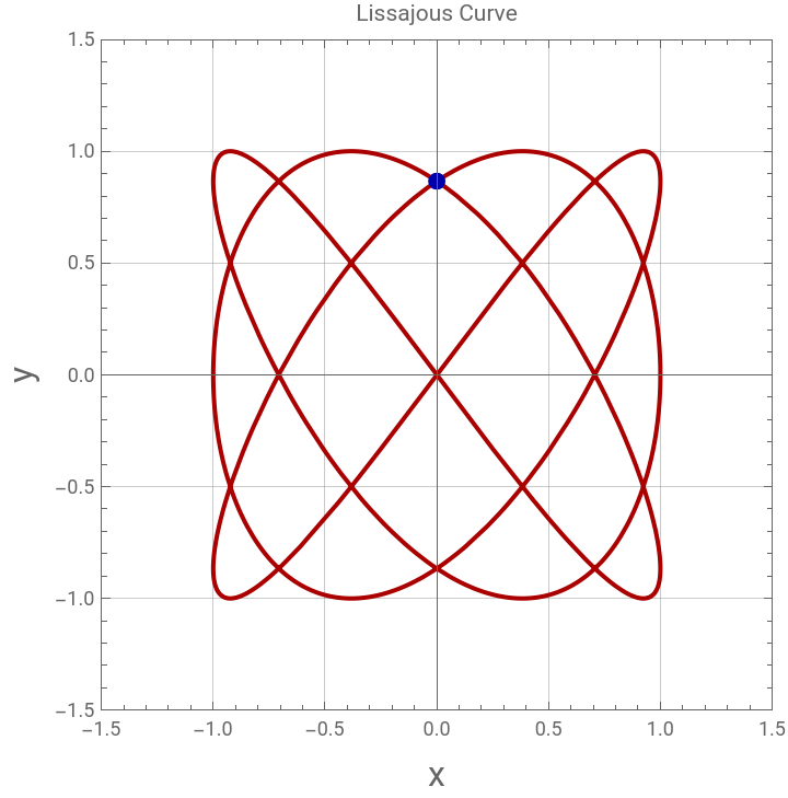
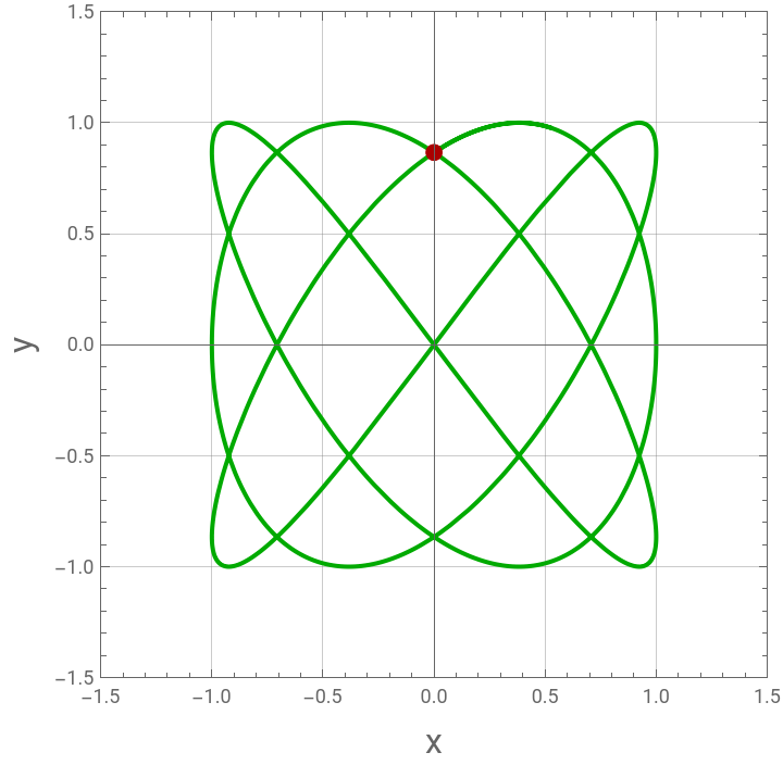
We compute the perimeter of a 3-by-4 multi-loop Lissajous structure using two different approaches: (1) the parametric definition of the Lissajous curve is defined and (2) Arc-length continuation (numerical differential approach).Method 1: Based on parametric definition of the Lissajous curveThe 3-by-4 multi-loop Lissajous structure is defined by: and The exact perimeter is given by: where: =0 and =2π.or equivalently Method 2: Arc-Length Continuation MethodThe second approach is based on the definition of arc length, where the perimeter is computed as the total length of a parametric curve.To do so, we use the following implict equation structure: and =1-Both calculations yield
x(t)=cos(3t)
y(t)=sin(4t)
P=+dt
t
1
∫
t
0
2
x
t
2
y
t
t
1
t
2
P=
2π
∫
0
9Sin+16
dt2
(3t)
2
Cos(4t)
x=4-3u
3
u
2
y
2
(8-8+1)
4
u
2
u
P=21.2372
Method based on parametric definition of the Lissajous curve
A=1.;(*amplitudeforx*)B=1.;(*amplitudefory*)a=3;(*frequencyforx*)b=4;(*frequencyfory*)delta=Pi/2;(*phase-shift*)x[t_]:=ASin[at+delta]y[t_]:=BSin[bt]
In[]:=
t1=t/.FindMinimum[{(x[t])^2,y[t]>=0},{t,7},AccuracyGoal->10][[2]]
Out[]=
6.80678
In[]:=
t0=t/.FindMinimum[{(x[t])^2,y[t]>=0},{t,0},AccuracyGoal->10][[2]]
Out[]=
0.523599
In[]:=
t1-t0(*commonperiodis2π*)
Out[]=
6.28319
In[]:=
%/Pi
Out[]=
2.
In[]:=
p=ParametricPlot[{x[t],y[t]},{t,t0,t1},PlotStyle->{Thick,Darker@Red},FrameLabel->{Style["x",16],Style["y",16]},PlotLabel->"Lissajous Curve",AspectRatio->1,PlotRange->{{-1.5,1.5},{-1.5,1.5}},Frame->True,GridLines->Automatic,AspectRatio->1];
In[]:=
Show[p,Graphics[{Darker@Blue,PointSize[0.025],Point[{x[t],y[t]}/.t->(t0+0.0)],Point[{x[t],y[t]}/.t->(t1-0.0)]}]]
Out[]=
In[]:=
dx[t_]:=D[x[t],t]dy[t_]:=D[y[t],t]ds[t_]:=Sqrt[dx[t]^2+dy[t]^2]L=NIntegrate[ds[t],{t,t0,t1},AccuracyGoal->20];Print["Perimeter = ",L]
Perimeter = 21.2372
In[]:=
(*alternativelyonecanusethefollowingcommand*)N[NIntegrate[Sqrt[9Sin[3t]^2+16Cos[4t]^2],{t,0,2Pi},WorkingPrecision->50,AccuracyGoal->30,PrecisionGoal->30,MaxRecursion->30],10]
Out[]=
21.23721523
Method based on arc - length continuation
In[]:=
Clear[x,y]
In[]:=
(*implicitequationstructure*)eq1=x[s]==4u[s]^3-3u[s];eq2=y[s]^2==1-(8u[s]^4-8u[s]^2+1)^2;
In[]:=
eq3=x'[s]^2+y'[s]^2==1(*auxiliaryequation*)
Out[]=
2
′
x
2
′
y
In[]:=
Solve[4u^3-3u==0,u]
Out[]=
{u0},u-,u
3
2
3
2
In[]:=
sol=FindRoot[{x==4u^3-3u,y^2==1-(8u^4-8u^2+1)^2}/.u->0.5Sqrt[3],{x,0.5},{y,0.5},AccuracyGoal->20]
Out[]=
{x-4.44089×,y0.866025}
-16
10
In[]:=
SOL=Quiet@First@NDSolve[{eq1,eq2,eq3,x[0]==0,y[0]==(y/.sol),u[0]==0.5Sqrt[3],x'[0]==0.01,y'[0]==0.0,u'[0]==-0.01},{x,y,u},{s,0,22},PrecisionGoal->15]
Out[]=
xInterpolatingFunction,yInterpolatingFunction,uInterpolatingFunction


In[]:=
p=ParametricPlot[{x[s],y[s]}/.SOL,{s,0,21.79},Frame->True,FrameLabel->{Style["x",16],Style["y",16]},PlotRange->{{-1.5,1.5},{-1.5,1.5}},GridLines->Automatic,PlotStyle->Darker@Green,ImageSize->Medium,AspectRatio->1];
In[]:=
Show[p,Graphics[{Darker@Red,PointSize[0.025],Point[{x[s],y[s]}/.SOL/.s->0.0],Point[{x[s],y[s]}/.SOL/.s->21.2372]}]]
Out[]=
In[]:=
P=N[s/.Quiet@FindRoot[(x[s]/.SOL)==0,{s,20},WorkingPrecision->20,AccuracyGoal->20],10]
Out[]=
21.23721538