Graphical Solution for a Multistage Continuous Feed-and-Bleed Ultrafiltration System
Authors: Housam Binous and Ahmed Bellagi
Graphical Solution for a Multistage Continuous Feed-and-Bleed Ultrafiltration System
Authors: Housam Binous and Ahmed Bellagi
Authors: Housam Binous and Ahmed Bellagi
Consider a continuous feed-and-bleed ultrafiltration multistage unit, using the gel polarization model for the limiting flux.
A protein solution is fed into an-stage continuous feed-and-bleed ultrafiltration system at a rate of 1 L/min. The feed enters at 10 g/L and the gel concentration can be taken to be 300 g/L. The mass transfer coefficient is in each stage and the corresponding area equals 0.9 .
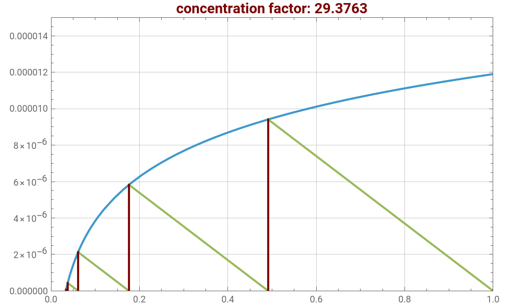
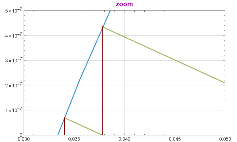
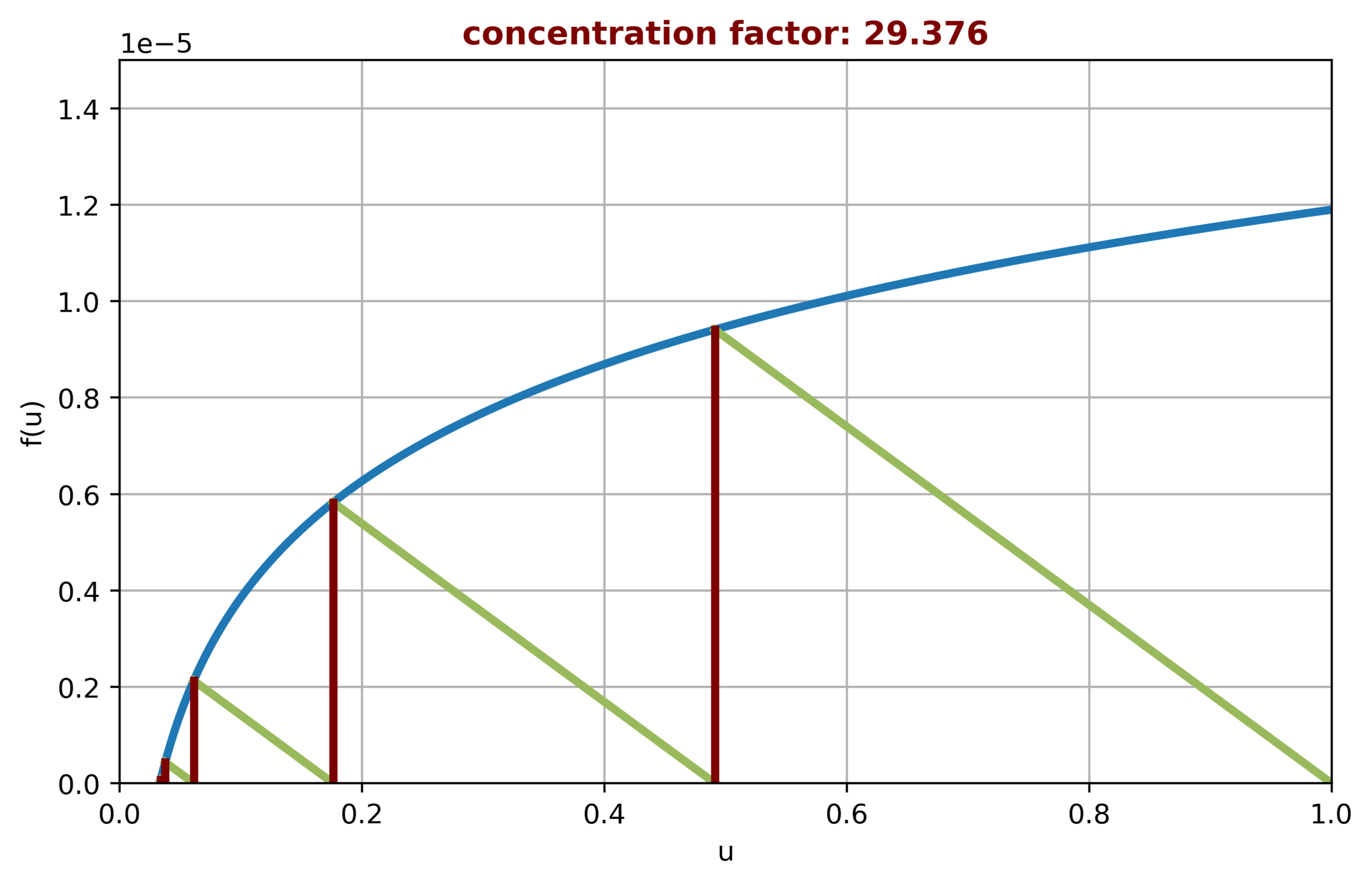
You can use a graphical approach developed by Foley [1] to obtain a value of the retentate concentration that exits the last membrane separation module. The blue curve is the flux curve, which can be thought of as an equilibrium line. The green lines trace the progress of the operation.
Here, we display this approach and give the value of the concentration factor (i.e. the ratio of the exit concentration to the inlet concentration). It is clear that beyond four stages, improvement of the concentration factor is negligible.
References:
[1] G. Foley, “Solution of Algebraic Equations in the Analysis, Design and Optimization of Continuous Ultrafiltration,” Chemical Engineering Education, 45(1), 2011 pp. 59–64.
A protein solution is fed into an
N
cg
3.5×m/s
-6
10
2
m
You can use a graphical approach developed by Foley [1] to obtain a value of the retentate concentration that exits the last membrane separation module. The blue curve is the flux curve, which can be thought of as an equilibrium line. The green lines trace the progress of the operation.
Here, we display this approach and give the value of the concentration factor (i.e. the ratio of the exit concentration to the inlet concentration). It is clear that beyond four stages, improvement of the concentration factor is negligible.
References:
[1] G. Foley, “Solution of Algebraic Equations in the Analysis, Design and Optimization of Continuous Ultrafiltration,” Chemical Engineering Education, 45(1), 2011 pp. 59–64.
In[]:=
Ns=5;(*numberofstagesNs*)x[0]=1;y[0]=0;(*steppingoffstages*)i=0;While[i<Ns+1,{x[i+1]=t/.FindRoot[1.1910^-5+3.510^-6Log[t]1.8510^-5(x[i]-t),{t,0.1}],y[i+1]=1.1910^-5+3.510^-6Log[x]/.xx[i+1],i++}];
In[]:=
x[5]
Out[]=
0.034041
In[]:=
plt1=Plot[1.1910^-5+3.510^-6Log[u],{u,0,1},PlotRange{{0,1},{0,1.510^-5}},FrameTrue,PlotStyleThick,GridLinesAutomatic,ImageSize{500,300},PlotLabelStyle["concentration factor: "<>ToString[1/x[5]],RGBColor[.49,0,0],Bold,14]];
In[]:=
plt2=Plot[1.1910^-5+3.510^-6Log[x],{x,0,1},PlotRange{{0,1},{0,1.510^-5}},FrameTrue,PlotStyleThick,GridLinesAutomatic,ImageSize{500,300},PlotLabelStyle["zoom",RGBColor[.6,.03,.6],Bold,14],PlotRange{{0.03,0.05},{0,510^-7}}];
In[]:=
Show[plt1,Graphics[{RGBColor[.6,.73,.36],Thick,Table[Line[{{x[i],0},{x[i+1],y[i+1]}}],{i,0,Ns-1}]}],Graphics[{RGBColor[.49,0,0],Thick,Table[Line[{{x[i],0},{x[i],y[i]}}],{i,0,Ns}]}]]
Out[]=
In[]:=
Show[plt2,Graphics[{RGBColor[.6,.73,.36],Thick,Table[Line[{{x[i],0},{x[i+1],y[i+1]}}],{i,0,Ns-1}]}],Graphics[{RGBColor[.49,0,0],Thick,Table[Line[{{x[i],0},{x[i],y[i]}}],{i,0,Ns}]}],PlotRange{{0.03,0.05},{0,510^-7}}]
Out[]=
Solution obtained with Python and corresponding code are given below.1- Graphical solution with Python
2- Corresponding Python code
import numpy as np
import matplotlib.pyplot as plt
from scipy.optimize import root_scalar
# number of stages
Ns = 5
# initialize arrays (size Ns+2)
x = np.zeros(Ns + 2)
y = np.zeros(Ns + 2)
x[0] = 1.0
y[0] = 0.0
# function definitions
def f_log(u):
return 1.19e-5 + 3.5e-6 * np.log(u)
# iterative loop
for i in range(Ns + 1):
# equation to solve:
# 1.19e-5 + 3.5e-6*log(t) = 1.85e-5*(x[i] - t)
def equation(t):
return 1.19e-5 + 3.5e-6 * np.log(t) - 1.85e-5 * (x[i] - t)
sol = root_scalar(equation, bracket=[1e-6, 1], method=’bisect’)
x[i + 1] = sol.root
y[i + 1] = f_log(x[i + 1])
# create smooth curve for plotting
u = np.linspace(1e-6, 1, 400)
v = f_log(u)
# main plot
plt.figure(figsize=(8, 4.8))
plt.plot(u, v, linewidth=3)
plt.xlim(0, 1)
plt.ylim(0, 1.5e-5)
plt.grid(True)
plt.xlabel(“u”)
plt.ylabel(“f(u)”)
plt.title(
f”concentration factor: {1/x[5]:.3f}”,
color=(0.49, 0, 0),
fontweight=”bold”)
# green diagonal-like lines
for i in range(Ns):
plt.plot(
[x[i], x[i + 1]],
[0, y[i + 1]],
color=(0.6, 0.73, 0.36),
linewidth=3)
# red vertical lines
for i in range(Ns + 1):
plt.plot(
[x[i], x[i]],
[0, y[i]],
color=(0.49, 0, 0),
linewidth=3)
plt.show()