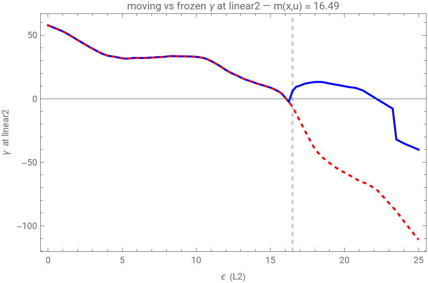
Robustness of neural networks is usually reported as one number: distance to the decision boundary. That hides which direction the boundary lies in and where inside the network the answer is actually formed. This essay measures both. A correctly classified MNIST digit is pushed along a ray through a pretrained LeNet, tracking a log-probability margin γ_l(ε;k) at every layer. Because the network is piecewise linear up to the logits, 'szeros — including the directional margin — are located exactly by bisection. An analytic, finite-difference-verified Jacobian feeds DeepFool, giving the isotropic margin and anisotropy ratio. Prediction depth, usually a fixed per-image score, is read as a function of from the same scan, so the two align by construction. Damage appears in depth long before the margin moves; adversarial and random directions differ by an order of magnitude; and past the crossing, the wrong answer crystallizes discontinuously rather than sliding in.
x+ϵu
γ
m(x,u)
m(x)
A(x,u)≥1
m(x,u)
m(x)
ϵ
Introduction
Introduction
A trained classifier reads a handwritten digit correctly. Random noise usually leaves the answer intact, while a far smaller perturbation, chosen carefully, overturns it. That distance defines robustness here, and it is larger than intuition suggests. The asymmetry is precise: classifiers that fall to worst case perturbations remain relatively robust to random ones, with random noise robustness scaling as roughly times the distance to the decision boundary, where is the input dimension[Fawzi et al ., 2016]. For a image, , so a random push must be nearly thirty times longer than an adversarial one. Robustness depends not only on how far the boundary lies, but on which way one moves.
d
d
2828
d784
The standard measure is therefore incomplete. The margin , the distance to the nearest boundary, compresses that geometry into one number; a point may sit close to the boundary along a few directions and far from it along most. It also ignores depth. A network assembles its answer layer by layer[Wolfram, 2023], and linear probes measure how much of it is present at each stage[Alain & Bengio, 2016], condensed into one per input quantity, the prediction depth[Baldock et al ., 2021]. Easy digits settle early; confusing ones require most of the network. Two rulers thus exist side by side: how far an input can be pushed before the answer breaks, and how deep that answer is formed. They have never been placed on a common axis. Neither has been used the way this essay requires.
m(x)
Prediction depth is defined and validated entirely on clean inputs[Baldock et al ., 2021], and subsequent work inherits that framing, treating it as a fixed difficulty score attached to an image rather than a quantity that responds to perturbation. Its behavior under a controlled push is, to our knowledge, unmeasured.
The margin has the opposite limitation. It is read at the output alone, and measurement stops once the answer flips. Ray based studies interpolate across the boundary and detect an inconsistency at the crossing[Bell et al ., 2025], and neighborhood analyses show that the boundaries surrounding adversarial points do not resemble those around benign ones[He et al ., 2018], yet neither resolves the crossing through depth, and neither asks what happens beyond it. The wrong answer has its own structure, how quickly and how deeply the network commits to it, and that structure has not been examined.
Both gaps close with a single construction. A correctly classified input is pushed along a ray , with a fixed unit direction and the distance traveled, measured in pixel units . At every layer we track the gap between the original class and its nearest competitor as grows. Because the network is piecewise linear up to the logits, this gap is exactly piecewise linear in , and its zeros are exact first passage distances located by bisection rather than estimated by gradient heuristics.
x+ϵu
u
ϵ
ϵ
ϵ
The first zero at the output is the directional margin , the distance at which the answer flips. It splits every ray into two regimes. Below it the network is still correct, and prediction depth becomes a function of rather than a fixed label: the lock in depth can be tracked as the correct answer dissolves. Above it the same instrument, re-referenced to the network's new class, measures how the wrong answer crystallizes, how quickly and how deeply the network commits to its mistake. Measurement therefore continues past the point where robustness studies ordinarily stop.
m(x,u)
ϵ
Two qualifications apply throughout. The probes here are logistic rather than NN, so what is measured is a variant of prediction depth, an alternative the original authors themselves considered[Baldock et al ., 2021]. And the isotropic margin used later as a reference is obtained by DeepFool with bisection, which yields an upper bound rather than the exact distance.
k
m(x)
This essay is organized as follows. Section 2 (Setup) fixes the network, the ray, and the two perturbation families, Gaussian and M-FGM, that bracket the gap between noise a network absorbs and noise built to break it. Section 3 (Methodology) constructs the two instruments read throughout: the linear probes and prediction depth, and the γ ladder from which the directional margin is the first zero. Sections 4 through 7 supply the machinery needed to go beyond a single direction: the analytic, finite-difference-verified Jacobian, DeepFool’s isotropic margin , and the anisotropy ratio that separates a distant boundary from a badly aimed ray. Section 8 is where the two rulers finally meet — depth and margin read together along one ray, on both sides of the crossing, showing the network’s answer erode and then the wrong answer crystallize. Section 9 repeats that reading across an ensemble of digits and directions to check that the single-ray anatomy generalizes. The Concluding Remarks draw out what the disagreement between depth and margin implies for how robustness should be measured, and sketch the natural extensions to deeper architectures, adversarially trained networks, and the re-crossing structure that a first-flip definition of robustness cannot see.
m(x,u)
m(x)
A(x,u)
Setup
Setup
In this analysis, we use LeNet, a simple convolutional neural architecture designed for handwritten digits recognition. The network drawn pretrained from the Wolfram Neural Net Repository on MNIST, a large dataset made of 28 × 28 pixel grayscale images of handwritten digits (0–9). Its layers are named by a short alias scheme (i.e. conv1, ramp1, pool1, …, linear2) giving a fixed tap list used throughout for probing intermediate representations. All geometry in this essay is measured at the logits, with the softmax deliberately excluded: this is what keeps the network piecewise linear up to the point of measurement, and it is what makes the exact, closed form arguments in later sections possible.
In[]:=
trainData=ResourceData["MNIST","TrainingData"];testData=ResourceData["MNIST","TestData"];net=NetModel["LeNet Trained on MNIST Data"];NetGraph[net]
Out[]=
NetGraph




A perturbation is applied along a ray: x+ϵu, where is a fixed unit direction (L2 norm, ) and is the distance traveled, measured in pixel units. The choice of linearity in is the standard choice in the adversarial robustness literature, it underlies FGSM-style attacks and the random direction robustness bounds of [Fawzi et al., 2016], and it is what makes distance along the ray directly comparable to a margin: moving in a straight line means the point at which the network’s answer changes is a single scalar, , rather than a path integral. Everything that follows (margin, ladder, prediction depth as a function of perturbation) is a functional of this one ray, evaluated as grows from 0.
The study uses two families of perturbation, selected to expose the gap between noise a network absorbs and noise that breaks it outright. Both enter the-ray identically and differ only in how is built. Random noise draws from a Gaussian and normalizes it. The resulting direction knows nothing about the image: it disturbs every pixel by a comparable amount, degrading informative and uninformative regions alike, and it carries no trace of what the network has learned. Adversarial noise inverts this. It is a targeted direction assembled from the network’s own gradients, and it spends its budget on precisely the pixels the classification rests upon.
The resulting asymmetry in robustness is geometric, not a property of the pixels. In high dimension a random direction is nearly orthogonal to the one direction along which the boundary sits close; the distance a random ray travels before crossing exceeds the true margin by roughly [Fawzi et al., 2016]. Related work makes the same point from the error-rate side: the error rate under Gaussian noise itself determines the distance to the boundary [Gilmer et al., 2019]. Robustness to noise therefore reflects the improbability of a blind direction finding the nearby boundary, not the boundary’s absence. A gradient-built direction finds it by construction. The two families bracket the same local geometry from opposite ends (typical and greedy) and reading both along a common ray is what makes them comparable.
′
x
u
∥u1
2
∥
ϵ
ϵ
ϵ
γ
ϵ
The study uses two families of perturbation, selected to expose the gap between noise a network absorbs and noise that breaks it outright. Both enter the
ϵ
u
u
The resulting asymmetry in robustness is geometric, not a property of the pixels. In high dimension a random direction is nearly orthogonal to the one direction along which the boundary sits close; the distance a random ray travels before crossing exceeds the true margin by roughly
d
Out[]=
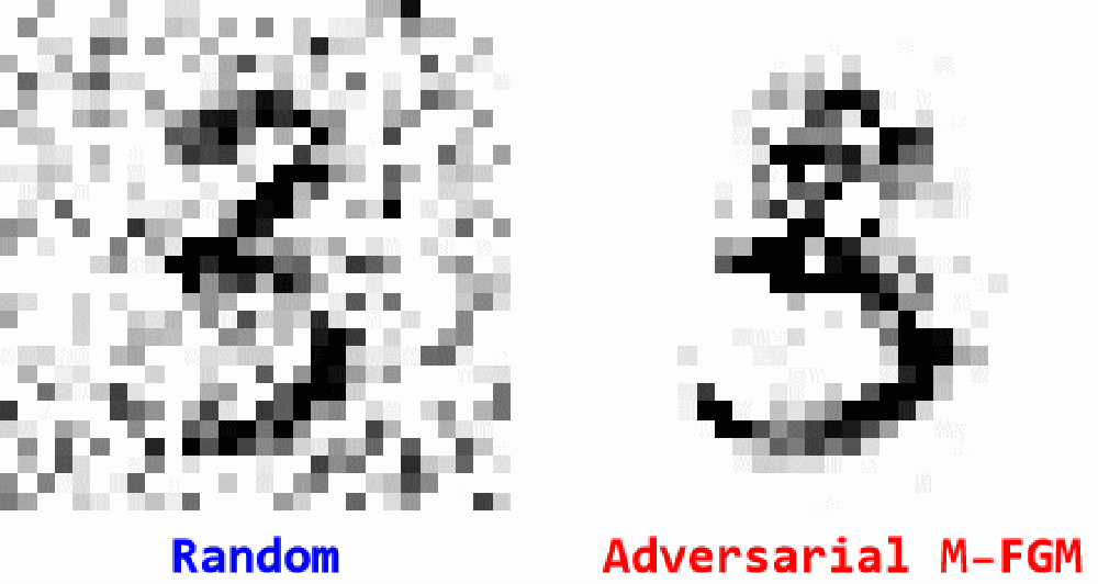
The Gaussian model is the simpler. A vector with i.i.d. standard-normal entries is normalized to unit length, sampling a direction uniformly from the unit sphere, independent of image and network alike.
u
G
z
∥z
∥
2
I
d
The adversarial model needs more deliberate design. The textbook choice is Fast Gradient Sign Method (FGSM) that is designed based on the sign of the cross-entropy gradient [Goodfellow et al., 2015]. FGSM is ill-suited here on two counts. It quantizes each pixel to ±1, ∼signLx,, discarding the relative magnitudes that identify which pixels matter, and the cross-entropy gradient attenuates as confidence grows, supplying little usable signal on a correctly and confidently classified digit, which is exactly where measurement starts. The ray instead requires a direction aligned with the quantity being measured, the logit margin. This variant, Margin-Fast Gradient Method (M-FGM) takes the normalized gradient of the margin between the base class and its nearest competitor, obtained in one backward pass.
u
FGSM
∇
x
y
u
M-FGM
z
∥z
∥
2
∇
x
f
competitor
f
label
It is the direction of steepest local decrease of the very function whose zero defines the margin, and it preserves magnitude information across pixels. Margin-based attack objectives of this kind are well established [Carlini & Wagner, 2017]; the departure from FGSM is what puts the adversarial ray on the same axis as the random one. M-FGM remains a single-step method: it commits to the gradient evaluated at and never revisits it. The natural next step in adversariality re-evaluates the linearization as the point moves, converging toward the closest boundary rather than the one the initial gradient implies (this is DeepFool [Moosavi-Dezfooli et al., 2016] will be introduced later) where it supplies the isotropic margin against which directional margins are referenced.
x
m(x)
Methodology
Methodology
Prediction depth
Prediction depth
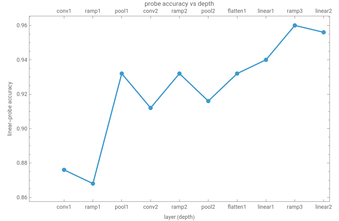
Prediction depth asks at what point in the network a decision has effectively been made. The construction has two parts: a way to read out what each layer “thinks”, and a rule for deciding when that readout has settled.The readout. Each tap in the layer list {conv1, ramp1, ... , linear2}, exposes an intermediate representation. tapFeatures extracts and flattens it, and trainLayerProbes fits one logistic-regression classifier per tap on clean MNIST features (Classify[…, Method → “LogisticRegression”]). The probe is deliberately linear, it cannot compute anything the representation has not already made linearly available, so its accuracy measures whether the class is readable at that depth, not whether it can be extracted with further nonlinear work. probeAccuracyVsDepth traces this across taps and gives the expected monotone rise — the representation becomes progressively more linearly separable with depth.
mnistTest=RandomSample[testData,250];acc=probeAccuracyVsDepth[net,probes,probeTaps,Keys[mnistTest],Values[mnistTest]];ListLinePlotValues[acc],
Out[]=
The rule. At a given input, probePredictions evaluates every probe in a single batched forward pass, producing a sequence of per-layer predicted classes. netClass gives the network’s own output class, final. Prediction depth is then the shallowest layer beyond which the probes never disagree with final again, , implemented as ta = LengthWhile[Reverse[seq], # === final], counting agreement from the deepest layer downward and subtracting from the layer count. The definition is a suffix condition, not a first-crossing condition: a probe agreeing early does not fix the depth if a later probe disagrees. What matters is where agreement begins and is never subsequently broken — the point at which the network has locked in its answer.
(PD(x)L-Number of trailing layers whose probe agrees with the network)
Out[]=

Two consequences of this design. If the deepest probe itself disagrees with the network, no suffix of agreement exists and the quantity is undefined; the implementation returns “NeverLocks” rather than a number. And because probes are trained once on clean features and then evaluated wherever they are asked, PD measured at a perturbed point x+ϵu reports where the clean representation is still recoverable — the probe is a fixed instrument, not one refit to the perturbed data. This is what makes PD comparable across and what allows it to be read against the margin on a common axis.
′
x
ϵ
γ Ladder
γ
Prediction depth reports a layer index, an integer that jumps. To see how a decision degrades along the ray, rather than merely when it flips, the discrete readout must be replaced by a continuous one. At each tap , the probe returns a distribution over classes. Define the margin of probe toward a reference class as the log-probability gap between and its strongest competitor,
l
l
k
k
γ
l
p
l
max
j≠k
p
l
The sign of is exactly the probe’s decision; > 0 when probe ℓ predicts k. The agreement indicator used by prediction depth is therefore not an independent construct but the sign of this quantity, (ϵ)[(ϵ;k)>0], and the PD staircase is a top-down scan over those signs. therefore, is the primitive; PD is a functional of it.
Two reference classes. The choice of carries ambiguity with it. It can be either fixed by the network’s prediction over the clean or perturbed input and both are covered by our implementation. First, , gamma fixes the reference as the network’s prediction of the clean input and it is denoted gammaFrozen and asks whether probe ℓ still holds the original class. Second, , the reference is the network’s prediction along the ray which varies as changes and it is denoted gammaMoving, which re-reads the network’s argmax at every grid point and asks whether probe agrees with the network now. In the regime where , the critical point at which the network fails to predict the input ( will be defined later as the margin ), both gammaFrozen and gammaMoving are equivalent (i.e. (ϵ)). Past the crossing they separate: the frozen ladder continues to measure erosion of the original class, while the moving ladder measures whether the layers have re-coordinated around the network’s new answer. Neither alone is sufficient — the frozen ladder cannot see re-coordination, the moving ladder cannot see what was lost — and their divergence point is precisely .
Piecewise linearity. The reason(ϵ) is worth defining at the logit tap, and the reason the crossing can be located exactly rather than approximated, is that the network is piecewise linear in its input up to the logits. Every operation from conv1 to linear2 is either affine (convolution, flatten, linear) or a fixed selection matrix (ramp, maxpool) once its gate is known. This is what §4 of the notebook makes explicit — the per-layer Jacobians are assembled by dispatch and multiplied into a single matrix. Within a linear region the gates are constant, so the logit vector along the ray is exactly affine in ,
γ
l
γ
l
a
l
γ
l
γ
Two reference classes. The choice of
k
k≡LeNet(x)
k
0
k(ϵ)≡LeNet(x+ϵu)
k
*
ϵ
l
ϵ<
*
ϵ
*
ϵ
m(x,u)
k
0
k
*
m(x,u)
Piecewise linearity. The reason
γ
l
(C,S(x),Π(x),,W)
P
flat
ϵ
f(x+ϵu)f(x)+ϵJ(x)u
and the logit-tap margin - , is an exactly linear function of with slope-. The softmax is excluded from the measurement for exactly this reason as it would destroy the affine structure that makes the statement exact. This yields a the -piecewise linearity of at the logit tap, that is made of a sequence of straight segments whose slopes change only when the ray crosses a gate boundary and the active linear region changes. The zeros of (ϵ) is therefore not a smooth curve’s root to be chased numerically, but the endpoint of a line segment; the grid-then-bisect scheme in probeCrossing is exact up to the tolerance, not an approximation to a curved crossing. The kinks in the ladder are themselves the record of how many linear regions the ray traversed — the same quantity that separates the one shot M-FGM direction from DeepFool’s iterated one. At the probe taps the picture is softer, since logistic regression composes a softmax with the affine readout, but the representation it reads remains piecewise linear in , and the kinks appear in the same places.
f
k
0
f
j
ϵ
(J(x)u)
k
0
(J(x)u)
j
ϵ
γ
γ
l
ϵ
Out[]=


DeepFool
DeepFool
Anisotropy: Directional vs Isotropic.
Anisotropy: Directional vs Isotropic.
Re-entry-aware prediction depth along the ray
Re-entry-aware prediction depth along the ray
◼
Median margin is 0.8-2.8 for M-FGM against 11.0-19.1 for Gaussian (disjoint ranges) no per-digit overlap. Gaussian/M-FGM ratio of medians is 8.3 at the median digit (5.2 on digit 1 to 21.5 on digit 4).
◼
Censoring averages 3.6% for M-FGM (max 8.2%) but 18.6% for Gaussian (max 61% on digit 8).
Concluding Remarks
Concluding Remarks
Acknowledgements
Acknowledgements
This project would not exist without the people who shaped it at every turn. Attending the Wolfram Summer Research Institute was a great opportunity That I’m grateful for. I would like to thank, Christian Pasquel for his mentorship and my group (Ahmet Erhan, Caden Lafollette, and Enrico Bottazzi) for many helpful discussions along the way. I would like to thank the program’s TAs (Nora Popescu and Julia Campolim) for their help with the technical implementations. I also thank Stephen Wolfram for suggesting the research direction that gave rise to this project.
References
References
1. G. Alain and Y. Bengio (2016), “Understanding Intermediate Layers Using Linear Classifier Probes,” arXiv preprint arXiv:1610.01644. https://arxiv.org/abs/1610.01644.
2. R. J. N. Baldock, H. Maennel and B. Neyshabur (2021), “Deep Learning Through the Lens of Example Difficulty,” Advances in Neural Information Processing Systems 34 (NeurIPS 2021), 10876–10889. https://arxiv.org/abs/2106.09647.
4. N. Carlini and D. Wagner (2017), “Towards Evaluating the Robustness of Neural Networks,” 2017 IEEE Symposium on Security and Privacy (SP), 39–57. https://arxiv.org/abs/1608.04644.
5. A. Fawzi, S.-M. Moosavi-Dezfooli and P. Frossard (2016), “Robustness of Classifiers: From Adversarial to Random Noise,” Advances in Neural Information Processing Systems 29 (NIPS 2016), 1632–1640. https://arxiv.org/abs/1608.08967.
6. N. Ford, J. Gilmer, N. Carlini and E. D. Cubuk (2019), “Adversarial Examples Are a Natural Consequence of Test Error in Noise,” Proceedings of the 36th International Conference on Machine Learning (ICML 2019), PMLR 97, 2280–2289. https://arxiv.org/abs/1901.10513.
7. I. J. Goodfellow, J. Shlens and C. Szegedy (2015), “Explaining and Harnessing Adversarial Examples,” 3rd International Conference on Learning Representations (ICLR 2015). https://arxiv.org/abs/1412.6572.
8. W. He, B. Li and D. Song (2018), “Decision Boundary Analysis of Adversarial Examples,” 6th International Conference on Learning Representations (ICLR 2018). https://openreview.net/forum?id=BkpiPMbA-.
9. Y. LeCun, L. Bottou, Y. Bengio and P. Haffner (1998), “Gradient-Based Learning Applied to Document Recognition,” Proceedings of the IEEE 86(11), 2278–2324. https://doi.org/10.1109/5.726791.
10. S. Wolfram (2023), “What Is ChatGPT Doing … and Why Does It Work?,” Stephen Wolfram Writings. https://writings.stephenwolfram.com/2023/02/what-is-chatgpt-doing-and-why-does-it-work/.
11. S.-M. Moosavi-Dezfooli, A. Fawzi and P. Frossard (2016), “DeepFool: A Simple and Accurate Method to Fool Deep Neural Networks,” 2016 IEEE Conference on Computer Vision and Pattern Recognition (CVPR), 2574–2582. https://arxiv.org/abs/1511.04599.
Wolfram Research (2019), “LeNet Trained on MNIST Data,” Wolfram Neural Net Repository. https://resources.wolframcloud.com/NeuralNetRepository/resources/LeNet-Trained-on-MNIST-Data.
Wolfram Research (2019), “LeNet Trained on MNIST Data,” Wolfram Neural Net Repository. https://resources.wolframcloud.com/NeuralNetRepository/resources/LeNet-Trained-on-MNIST-Data.
AI Disclosure
AI Disclosure
Generative AI tools were used in this project for literature search, brainstorming and conceptualization, paraphrasing, and code optimization and debugging. All mathematical arguments, pipeline design, and interpretation of results are the author’s own, and all numerical results were produced by the code in this notebook rather than by any AI tool. All code and written content was reviewed, understood, and approved by the author.
CITE THIS NOTEBOOK
CITE THIS NOTEBOOK
The Shape of a Wrong Answer: Directions in Neural Robustness
by Mohamed H Gouda
Wolfram Community, STAFF PICKS, July 16, 2026
https://community.wolfram.com/groups/-/m/t/3763419
by Mohamed H Gouda
Wolfram Community, STAFF PICKS, July 16, 2026
https://community.wolfram.com/groups/-/m/t/3763419