From the fundamental theorem of calculus, we have ,if we tolerate the abuse of as both the independent variable in and the variable of integration. If, for a given function and some function , we have =F(x,y), or equivalently, , and let =f(), then is a solution of the equation . In other words, it is a fixed point of the so-called Picard iteration: =+F(x,)x.The sequence may start with an arbitrary continuous function =(x). By the Picard-Lindelöf theorem, for a suitably nice function , the sequence of functions (x) converges to a differentiable function such that is a solution to the differential equation =F(x,y).
f(x)=f()+f'(x)x
x
0
x
∫
x
0
x
f(x)
y=f(x)
F(x,y)
dy
dx
f'(x)=F(x,f(x))
y
0
x
0
y=f(x)
y=+F(x,y)x
y
0
x
∫
x
0
y
n+1
y
0
x
∫
x
0
y
n
y
1
y
1
F
y
n
f(x)
y=f(x)
dy
dx
To illustrate the numerical behavior of this sequence, I chose to approximate over the interval using the Picard iteration with and =1 and chose the trapezoidal rule to approximate the indefinite integral.
y=
x
e
[0,1]
F(x,y)=y
y
0
Context and motivation
Context and motivation
I was searching for introductory examples of numerical routines for a course in Numerical Analysis. Day One, aside from introducing the course, we looked at fixed-point iterations for approximating numbers, to observe concepts we will study analytically: error, convergence, lack of convergence. On Day Two, I wanted an example to introduce discrete approximations of functions; additionally, to examine some mathematical notions to be introduced or reviewed: derivatives, integrals, norms, Taylor series. For the motivation for the “TDA,” see Trefethen, Ten Digit Algorithms, https://people.maths.ox.ac.uk/trefethen/tda05.pdf (2005): “Ten digits, five seconds, and just one page.”
Simple, ten-digit example: Exp[x] over [0, 1]
Simple, ten-digit example: Exp[x] over [0, 1]
TDA: ~10 lines of code, <1/10 second, >10 digits accuracy
TDA: ~10 lines of code, <1/10 second, >10 digits accuracy
In[]:=
(*" Restrictions: Assumes regular partition into Length[y]-1 intervals Approximates y0 + \int_0^x y dx, 0<=x<=1 The number y0 starts the list of y values (input and out) "*)trapRule[]=y|->PrependFirst@y+Accumulate,First@y;
Most[y]+Rest[y]
2
1
Length[y]-1
Ten-digit computation (error ):
<
1
2
-10
10
Block[{x,n=16},x=Subdivide[0.,1.,2^n];(*2^16intervals*)approx10=Nest[trapRule[],1+x(*initialfunctiony_1*),12];(*iterate12times*)Norm[(approx10-Exp[x])/Exp[x],Infinity](*maxabs.rel.diff.invalues*)]//AbsoluteTiming(*Output:{time,error}(MacbookProM4Max)*)
Out[]=
{0.010265,1.63449×}
-11
10
The basic algorithm is lovely and succinct for :
y()=1
x
0
Nest[trapRule[],1+{,…,},k]
x
0
x
N
Visualization of the result
Visualization of the result
With{exp=Exp[Subdivide[0.,1.,2^8]],(*1+2^8=257points*)downsample=approx10[[;;;;2^8]]},(*1+2^16/2^8=257points*)ListLinePlot[{exp,downsample},PlotStyle->{Black,Dashed},DataRange->{0,1},PlotLabel->"Exp[x], approx"(*,ImageSize->{Automatic,200}*),PlotLegends->Placed[{"Exp[x]","approx"},{Right,Bottom}],ImageSize->{Automatic,200}],ListLinePlot,DataRange->{0,1},PlotLabel->"Rel. Error",ImageSize->{Automatic,200}//Row
downsample-exp
exp
Out[]=
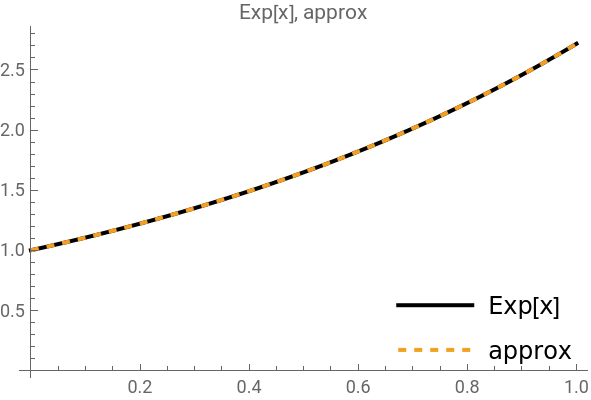
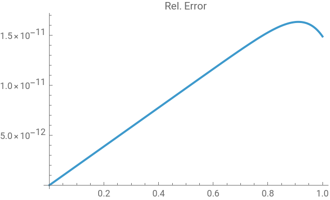
Visualization of convergence
Visualization of convergence
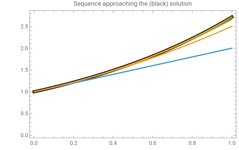
One can see the curves of the first few iterations approach the graph of before the rest more or less coincide with it. See the section “Computational comparison of convergence with theoretical bounds” further down for a view of the rate of convergence.
x
e
Block[{x,downsample},x=Subdivide[0.,1.,2^16];data=NestList[trapRule[],1+x,12];downsample=#[[;;;;Max[1,Floor[Length[#]/256]]]]&/@data;With[{plotOpts={DataRange->{0,1},Joined->True,Frame->True,ImageSize->400,ImagePadding->{{50,5},{20,5}},PlotLegends->Automatic}},Show[ListPlot[Exp[x],PlotStyle->{AbsoluteThickness[5],Black},plotOpts],ListPlot[downsample,plotOpts],PlotLabel->"Sequence approaching the (black) solution"]]]
Out[]=


Small data example:
Small data example:
The first row below the top line is the initial function =1+x, from which it is easy to deduce . The last row contains the values of for comparison. Eventually, the pointwise values overshoot the values of . And in the TDA above, the error was positive. Questions for reflection: Does that always happen that the error is eventually positive? Can the amount of overshoot be quantified (estimated or bounded)?
y
1
x
x
e
x
e
Block[{x,n=3},x=Subdivide[0.,1.,2^n];(*2^3=8intervals*)data8=NestList[trapRule[],1+x(*initialfunctiony_1*),5];(*iteratefivetimes*)Grid[(*displaytableofresults*)Join[Join[(*labels*){{HoldForm[x]}},Array[{Subscript[y,#]}&,Length@data8],{{HoldForm[E^x]}}],Join[(*values*){x},data8,{Exp[x]}],2],Dividers->{{2->True},{2->True,-2->True}},Alignment->"."]]
Beyond ten digits
Beyond ten digits
Extend to thirteen digits (again no negative errors):
Block[{x,n=21,error},x=Subdivide[0.,1.,2^n];(*2^21≈2*10^6intervals*)approx13=Nest[trapRule[],1+x(*initialfunctiony_1*),15];(*iterate15times*)error=approx13-Exp[x];Echo[Counts[Sign[error]],"Signs of errors:"];Norm[error/Exp[x],Infinity](*maxrel.error*)]//AbsoluteTiming
The approximation doesn’t really improve substantially from here:
The roundoff plateau
The roundoff plateau
Analysis of the Picard sequence
Analysis of the Picard sequence
An exact Picard iteration
An exact Picard iteration
There is a clear pattern. Question: How can we use induction to give a complete proof?
Bounding the error
Bounding the error
Convergence by computational induction
Convergence by computational induction
FindSequenceFunction[] performs computational induction, attempting to infer a general formula from a few terms of a sequence.
We obtain the formula for the error bound, and its limit is zero.
Analysis of the discrete Picard iteration
Analysis of the discrete Picard iteration
The discrete recurrence system
The discrete recurrence system
The fixed may be determined by solving the system:
Convergence
Convergence
Dependence on the step size of the trapezoidal rule
Dependence on the step size of the trapezoidal rule
The following shows the error in the trapezoidal rule to decrease as the square of the step size in the subdivision of the interval:
Independence of convergence on starting function
Independence of convergence on starting function
One consequence of the analysis of the convergence of the Picard iteration is that no matter what bounded function one starts the sequence with, the sequence converges to the exponential function. The smoothing of the random fluctuations with each integration is apparent. The downward spikes in the error, both above and below, usually come from the solution crossing the exponential graph.
Computational comparison of convergence with theoretical bounds
Computational comparison of convergence with theoretical bounds
Addendum: More context and motivation
Addendum: More context and motivation
There are lots of reason why I got excited by this example. A few:
◼
Discrete approximation of continuous processes (functions of a continuous variable, integration) actually works.
◼
The algorithm is easy to understand. (Its convergence is less easy, but….)
◼
Convergence is visible and impressive.
◼
Convergence is pretty good even with a small number of sample points, making it feasible to inspect the data.
◼
The natural exponential function is a somewhat difficult function to deal with at the pre-calculus level, but approximating it appears simple in this context.
◼
The trapezoidal rule is an elementary numerical algorithm, sometimes taught in intro calculus and recently discovered to date from as far back as the Babylonians; see Ossendrijver, https://www.science.org/content/article/math-whizzes-ancient-babylon-figured-out-forerunner-calculus-2 (2016).
Another note on context: The numerical analysis course and differential equations course may be taken independently at my institution. Consequently, I do not stress the role of the Picard iteration in differential equations or the rather close connection of the method here to the trapezoidal rule in numerical differential equations.
CITE THIS NOTEBOOK
CITE THIS NOTEBOOK
Numerical Picard iteration with trapezoidal quadrature for initial value problems
by Michael Rogers
Wolfram Community, STAFF PICKS, February 13, 2026
https://community.wolfram.com/groups/-/m/t/3639273
by Michael Rogers
Wolfram Community, STAFF PICKS, February 13, 2026
https://community.wolfram.com/groups/-/m/t/3639273