Temperature Distribution and Residue Curve Map for Isopropyl Acetate Chemistry at 1 atm
Temperature Distribution and Residue Curve Map for Isopropyl Acetate Chemistry at 1 atm
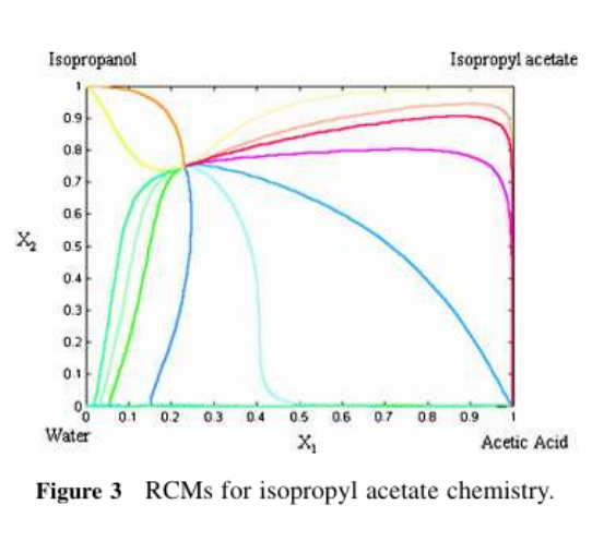
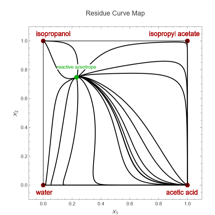
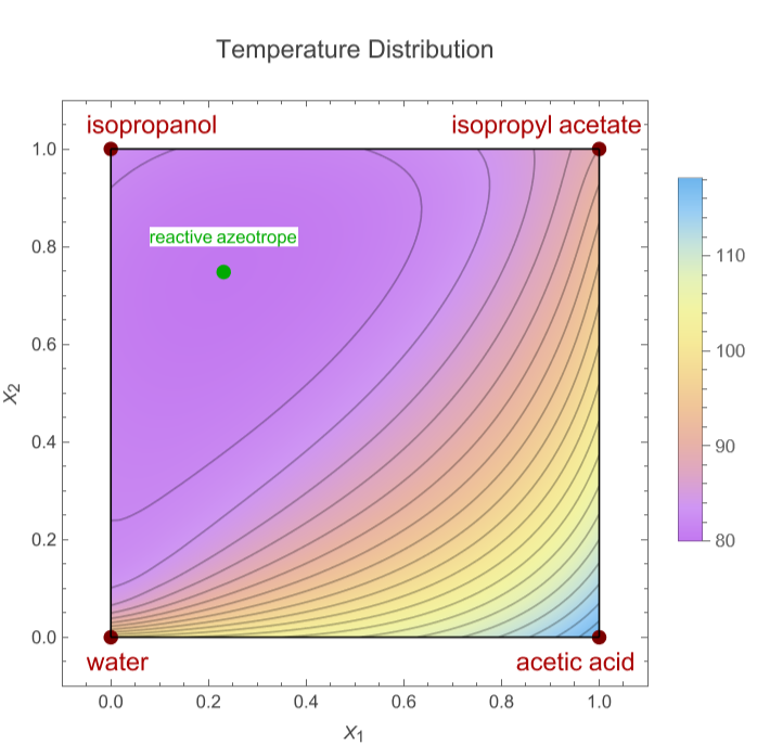
The system considered is the esterification of acetic acid with isopropanol to produce isopropyl acetate and water:COOH+CH(OH)⇌+O.Again, I plot the residue curve map.There is a reactive azeotrope corresponding to =0.231 and =0.748. This reactive azeotrope is an unstable node (indicated by a green dot in the magenta region). In addition, there are two nonreactive binary azeotropes. The first is between isopropanol and water, while the other is between isopropanol and isopropyl acetate. Both nonreactive azeotropes are saddle points. Isopropyl acetate and water are two saddle points while acetic acid (light blue region) and isopropanol are two stable nodes.The axes labels are and , with the independent liquid transformed compositions given by: =+ and =+, where is the liquid mole fraction of component and isopropyl acetate is the reference component.The code also displays the iso-temperature curves where the temperature is in °C.Finally, Particle Swarm Optimization (PSO) is used to fetch the transformed compositions of the minimum and maximum bubble temperatures points.
CH
3
CH
3
CH
3
CH
3
COOCH()
CH
3
2
H
2
X
1
X
2
X
1
X
2
X
1
x
aceticacid
x
isopropylacetate
X
2
x
isopropanol
x
isopropylacetate
x
A
A
In[]:=
G[i_,t_]:=Exp(tau[j,i,t]Ga[j,i,t]x[j])(Ga[l,i,t]x[l])+(Ga[l,j,t]x[l])tau[i,j,t]-(tau[r,j,t]Ga[r,j,t]x[r])(Ga[l,j,t]x[l])/.x[1]x1[t]/.x[2]x2[t]/.x[3]x3[t]/.x[4]x4[t];
4
∑
j=1
4
∑
l=1
4
∑
j=1
Ga[i,j,t]x[j]
4
∑
l=1
4
∑
r=1
4
∑
l=1
In[]:=
Ga[i_,j_,t_]:=Exp[-ai[i,j]tau[i,j,t]];
In[]:=
tau[i_,j_,t_]:=g[i,j]/(RT[t]);
In[]:=
g[1,1]=0;g[2,1]=81.3926;g[3,1]=154.7885;g[4,1]=842.6081;g[1,2]=-281.4482;g[2,2]=0;g[3,2]=140.0972;g[4,2]=1655.2550;g[1,3]=141.0082;g[2,3]=269.9609;g[3,3]=0;g[4,3]=1270.2036;g[1,4]=-219.7238;g[2,4]=39.8541;g[3,4]=1165.709;g[4,4]=0;
In[]:=
ai[1,1]=0;ai[2,1]=0.3048;ai[3,1]=0.3014;ai[4,1]=0.2997;ai[1,2]=0.3048;ai[2,2]=0;ai[3,2]=0.3009;ai[4,2]=0.3255;ai[1,3]=0.3014;ai[2,3]=0.3009;ai[3,3]=0;ai[4,3]=0.3300;ai[1,4]=0.2997;ai[2,4]=0.3255;ai[3,4]=0.3300;ai[4,4]=0;
In[]:=
Psat[i_,t_]:=Exp[(Aa[i]+Ba[i]/(T[t]+Ca[i]))];Aa[1]=23.3618;Aa[2]=25.3358;Aa[3]=21.7798;Aa[4]=23.4776;Ba[1]=-4457.83;Ba[2]=-4628.96;Ba[3]=-3307.73;Ba[4]=-3984.92;Ca[1]=-14.699;Ca[2]=-20.514;Ca[3]=-39.485;Ca[4]=-39.724;
In[]:=
Ksym[t_]:=10^(-12.5454+3166/(T[t]));
In[]:=
Keq1=8.7;
In[]:=
y2[t_]:=Chop[Psat[2,t]G[2,t]x2[t]/((2(1-y1[t]+Sqrt[(1+4Ksym[t]Py1[t](2-y1[t]))]))/((2-y1[t])(1+Sqrt[(1+4Ksym[t]Py1[t](2-y1[t]))])))1/P];y3[t_]:=Chop[Psat[3,t]G[3,t]x3[t]/((2(1-y1[t]+Sqrt[(1+4Ksym[t]Py1[t](2-y1[t]))]))/((2-y1[t])(1+Sqrt[(1+4Ksym[t]Py1[t](2-y1[t]))])))1/P];
In[]:=
Y1[t_]:=Chop[y1[t]+y3[t]];Y2[t_]:=Chop[y2[t]+y3[t]];
In[]:=
x4[t_]:=1-x1[t]-x2[t]-x3[t];
In[]:=
R=1.987;P=1.01310^5;
In[]:=
sol=.
In[]:=
sol[p1_,p2_]:=Quiet[NDSolve[{X1[t]x1[t]+x3[t],X2[t]x2[t]+x3[t],G[1,t]G[2,t]x1[t]x2[t]-G[3,t]G[4,t]x3[t]x4[t]/Keq10,PPsat[1,t]G[1,t]x1[t]/((1+Sqrt[(1+4Ksym[t]Psat[1,t])])/(1+Sqrt[(1+4Ksym[t]Py1[t](2-y1[t]))]))+Psat[2,t]G[2,t]x2[t]/((2(1-y1[t]+Sqrt[(1+4Ksym[t]Py1[t](2-y1[t]))]))/((2-y1[t])(1+Sqrt[(1+4Ksym[t]Py1[t](2-y1[t]))])))+Psat[3,t]G[3,t]x3[t]/((2(1-y1[t]+Sqrt[(1+4Ksym[t]Py1[t](2-y1[t]))]))/((2-y1[t])(1+Sqrt[(1+4Ksym[t]Py1[t](2-y1[t]))])))+Psat[4,t]G[4,t]x4[t]/((2(1-y1[t]+Sqrt[(1+4Ksym[t]Py1[t](2-y1[t]))]))/((2-y1[t])(1+Sqrt[(1+4Ksym[t]Py1[t](2-y1[t]))]))),y1[t]Psat[1,t]G[1,t]x1[t]/((1+Sqrt[(1+4Ksym[t]Psat[1,t])])/(1+Sqrt[(1+4Ksym[t]Py1[t](2-y1[t]))]))1/P,D[X1[t],{t,1}]-X1[t]+Y1[t],D[X2[t],{t,1}]-X2[t]+Y2[t],X1[0]p1,X2[0]p2,T[0]360,y1[0]0.0000025,x1[0]0.00867394,x2[0]0.308674,x3[0]==0.191326},{x1[t],x2[t],x3[t],y1[t],X1[t],X2[t],T[t]},{t,-80,80}]];
In[]:=
rcm[{p1_,p2_}]:=Quiet@ShowParametricPlotEvaluate[{X1[t],X2[t]}/.sol[p1,p2]],{t,-40,40},,
In[]:=
tbli=;
In[]:=
RCM=Show[Table[rcm[tbli[[i]]],{i,1,Length@tbli}],PlotLabel->Style["\nResidue Curve Map\n",14]]
Out[]=
In[]:=
LaunchKernels[]
Out[]=
KernelObject

In[]:=
tbl=Parallelize@Table[{{i,j},T[t]/.Quiet[FindRoot[{ix1[t]+x3[t],jx2[t]+x3[t],G[1,t]G[2,t]x1[t]x2[t]-G[3,t]G[4,t]x3[t]x4[t]/Keq10,PPsat[1,t]G[1,t]x1[t]/((1+Sqrt[(1+4Ksym[t]Psat[1,t])])/(1+Sqrt[(1+4Ksym[t]Py1[t](2-y1[t]))]))+Psat[2,t]G[2,t]x2[t]/((2(1-y1[t]+Sqrt[(1+4Ksym[t]Py1[t](2-y1[t]))]))/((2-y1[t])(1+Sqrt[(1+4Ksym[t]Py1[t](2-y1[t]))])))+Psat[3,t]G[3,t]x3[t]/((2(1-y1[t]+Sqrt[(1+4Ksym[t]Py1[t](2-y1[t]))]))/((2-y1[t])(1+Sqrt[(1+4Ksym[t]Py1[t](2-y1[t]))])))+Psat[4,t]G[4,t]x4[t]/((2(1-y1[t]+Sqrt[(1+4Ksym[t]Py1[t](2-y1[t]))]))/((2-y1[t])(1+Sqrt[(1+4Ksym[t]Py1[t](2-y1[t]))]))),y1[t]Psat[1,t]G[1,t]x1[t]/((1+Sqrt[(1+4Ksym[t]Psat[1,t])])/(1+Sqrt[(1+4Ksym[t]Py1[t](2-y1[t]))]))1/P},{x1[t],0.01},{x2[t],0.01},{x3[t],0.01},{T[t],350},{y1[t],0.5},MaxIterations10000]//Chop]},{j,0,1,0.05},{i,0,1,0.05}];(*maytakeafewminutes*)
In[]:=
tblf=Flatten[tbl,1];
In[]:=
f=Interpolation[tblf];
pltD2=ShowDensityPlotf[xs,ys]-273.15`,{xs,0,1},{ys,0,1},,Graphics[{Style[Text["water",{-0.05`,-0.05`},{-1,0}],Darker[Red],14],Style[Text["isopropanol",{-0.05`,1.05`},{-1,0}],Darker[Red],14],Style[Text["isopropyl acetate",{1.05`,1.05`},{0.8`,0}],Darker[Red],14],Style[Text["acetic acid",{1.05`,-0.05`},{0.8`,0}],Darker[Red],14],Style[Text["reactive azeotrope",{0.231`,0.82`},{0,0}],Darker[Green],10,BackgroundWhite],RGBColor[0.49`,0,0],PointSize[0.025`],Point[{1,0}],Point[{1,1}],Point[{0,1}],Point[{0,0}],Darker[Green],Point[{0.231`,0.748`}]}]
Out[]=
Final checks. The transformed compositions of the reactive azeotrope is :
Boiling point of reactive azeotrope
Acetic acid boiling point
Seeking loci of highest and lowest boiling point nodes using PSO - one gets acetic acid (117.79°C) and the reactive azeotrope (79.71°C)
2D problem
Upper and lower bounds for the search domain
PSO parameters
For reader to reproduce exactly the PSO results found below
Clip each column of a matrix against its own scalar bound
PSO Optimizer
PSO convergence plot
PSO convergence plot
Temperature Distribution and Residue Curve Map for Methyl Acetate Chemistry at 1 atm
Temperature Distribution and Residue Curve Map for Methyl Acetate Chemistry at 1 atm
Final checks. The transformed compositions of the azeotrope is:
Boiling point of methanol-methyl acetate positive azeotrope
Acetic acid boiling point
Seeking loci of highest and lowest boiling point nodes using PSO - one gets acetic acid (117.79°C) and the positive azeotrope between methanol and methyl acetate (53.51°C)
2D problem
Upper and lower bounds for the search domain
PSO parameters
For reader to reproduce exactly the PSO results found below
Clip each column of a matrix against its own scalar bound
PSO Optimizer
PSO convergence plot
PSO convergence plot
Temperature Distribution and Residue Curve Map for Ethyl Acetate chemistry at 1 atm
Temperature Distribution and Residue Curve Map for Ethyl Acetate chemistry at 1 atm
Final checks. The transformed compositions of the two azeotropes are :
Boiling point of ethanol-ethyl acetate positive azeotrope
Boiling point of ethanol-water positive azeotrope
Acetic acid boiling point
2D problem
Upper and lower bounds for the search domain\
PSO parameters
For reader to reproduce exactly the PSO results found below
Clip each column of a matrix against its own scalar bound
PSO Optimizer
Seeking loci of highest and lowest boiling point nodes using PSO - one gets acetic acid (117.79°C) and the positive azeotrope between ethanol and ethyl acetate (72.17°C)
PSO convergence plot
PSO convergence plot
References
References
[1] M. F. Doherty and M. F. Malone, Conceptual Design of Distillation Systems, New York: McGraw-Hill, 2001.
[2] H. Binous, Residue curve map for homogeneous reactive quaternary mixtures, Comput. Appl. Eng. Educ., 15 (2007), pp. 73-77.
https://doi.org/10.1002/cae.20099
https://doi.org/10.1002/cae.20099
CITE THIS NOTEBOOK
CITE THIS NOTEBOOK
Temperature distribution and residue curve maps for acetate ester systems at 1 atm
by Housam Binous
Wolfram Community, STAFF PICKS, August 2, 2026
https://community.wolfram.com/groups/-/m/t/3772298
by Housam Binous
Wolfram Community, STAFF PICKS, August 2, 2026
https://community.wolfram.com/groups/-/m/t/3772298