We study a first-order series (consecutive) reaction A → B → C carried out at steady state in a single continuous stirred-tank reactor (CSTR). B is the desired product and C is an over-reaction/side product formed from B.
Kinetics: both steps are modeled as first order with Arrhenius-type rate constants:
k1(T) = A1 Exp[-E1/(Rgas T)] for A → B (desired step)
k2(T) = A2 Exp[-E2/(Rgas T)] for B → C (side step)
The side step has the higher activation energy (E2 > E1), so it is more sensitive to temperature than the desired step -- raising T speeds up A → B but speeds up B → C even faster.
CSTR performance: for the given residence time τ and temperature T, the conversion of A and the selectivity toward B are modeled as
XA(τ,T) = k1(T) τ / (1 + k1(T) τ ) (fraction of A converted)
SB(τ,T) = 1 / (1 + k2(T) τ ) (probability a B molecule has not yet reacted onward to C)
SB is a compact first-order "survival fraction" proxy for selectivity, not the full algebraic solution of a coupled A/B/C component balance (which would also depend on XA and k1). It is a reasonable simplification for exploring the qualitative conversion/selectivity trade-off studied here.
Design variables: residence time τ and reactor temperature T.
Objectives:
Conversion XA and selectivity SB both increase in ways that conflict with each other -- longer residence time and higher temperature raise conversion XA but erode selectivity SB, because more of the B that has already formed gets a chance to react onward to C.
The goal of this notebook is to (1) map out that trade-off as a Pareto front (the set of designs where XA cannot be improved without sacrificing SB, or vice versa),
and (2) pick a single balanced compromise design from that front.
Kinetics and CSTR Model
In[]:=
(*Universalgasconstant,usedinsidetheArrheniusexpressionsbelow*)Rgas=8.314;(*J/mol/K*)(*Pre-exponentialfactorandactivationenergyforthedesiredstepA→B*)A1=5*10^4;E1=45000;(*desiredstepA→B*)(*Pre-exponentialfactorandactivationenergyforthesidestepB→C;*)(*noteE2>E1,sothisstepismoretemperature-sensitivethanthefirst*)A2=5*10^7;E2=75000;(*sidestepB→C,moreT-sensitive*)(*Arrheniusrateconstantsk1(T),k2(T),asfunctionsoftemperatureT[K]*)k1[T_]:=A1*Exp[-E1/(Rgas*T)];k2[T_]:=A2*Exp[-E2/(Rgas*T)];
In[]:=
(*CSTRperformanceequations*)(*Steady-stateconversionofAinaCSTR,asafunctionofresidence*)(*timeτandtemperatureT:XA=k1*τ/(1+k1*τ)*)XA[τ_,T_]:=k1[T]*τ/(1+k1[T]*τ);(*SelectivitytowardthedesiredproductB:modeledastheprobability*)(*thataBmoleculehasnotyetreactedfurthertoC,i.e.thefirst-*)(*order"survival fraction"SB=1/(1+k2*τ)*)SB[τ_,T_]:=1/(1+k2[T]*τ);
Sampling the Design Space
In[]:=
(*Buildthedesigngrid*)(*Residencetimeτ,sweptfrom0.05to80instepsof0.1*)τVals=Table[τ,{τ,0.05,80,0.1}];(*TemperatureT,sweptfrom300Kto650Kinstepsof2K*)TVals=Table[T,{T,300,650,2}];
In[]:=
(*Forevery(τ,T)combinationonthegrid,evaluatebothobjectives*)(*andkeepthedesignvariablesalongsidethem:{XA,SB,τ,T}.*)points=Flatten[Table[{XA[τ,T],SB[τ,T],τ,T},{T,TVals},{τ,τVals}],1];
Extracting the Pareto Front
Both objectives (XA and SB) are to be maximized, so a design point is Pareto-optimal (non-dominated) if no other grid point has both a higher XA and a higher SB. This is found efficiently with the classic "skyline" algorithm for two objectives: sort all points by XA descending, then sweep through them and keep a point only when its SB exceeds the best SB seen so far among all higher-XA points. Any point that fails this test is dominated by some earlier (higher-XA, higher- or equal-SB) point and is discarded.
In[]:=
(*Step1:sortallgridpointsbyconversionXA,descending*)sorted=SortBy[points,-#[[1]]&];
In[]:=
(*Step2:sweepthroughthesortedlist,keepingapointonlyifits*)(*selectivitySBisanew"best so far"amongallpointswithequal*)(*orhigherconversionseenuptothispointinthesweep*)frontier={};maxSB=-Infinity;Do[If[pt[[2]]>maxSB,AppendTo[frontier,pt];maxSB=pt[[2]]],{pt,sorted}];(*re-sorttheretainedfrontierpointsbyXAascendingforplotting*)frontier=SortBy[frontier,First];(*sortbyXAascendingforplotting*)
In[]:=
(*ReporthowmuchthegridwasthinneddownbytheParetofilter,and*)(*printacoarsesampleofthefrontier(about15evenly-spacedrows)*)Print["Grid points: ",Length[points]];Print["Pareto-optimal points: ",Length[frontier]];
Grid points: 140800
Pareto-optimal points: 8413
In[]:=
TableForm[frontier[[1;;-1;;Max[1,Floor[Length[frontier]/15]]]],TableHeadings->{None,{Style["XA",Darker@Red],Style["SB",Darker@Red],Style["τ",Darker@Red],Style["T",Darker@Red]}}]
Out[]//TableForm=
XA | SB | τ | T |
0.0000365128 | 1. | 0.05 | 300 |
0.0385808 | 0.99976 | 54.95 | 300 |
0.0809143 | 0.999282 | 75.45 | 308 |
0.155229 | 0.997509 | 73.35 | 322 |
0.276561 | 0.991781 | 75.75 | 336 |
0.44193 | 0.972791 | 75.45 | 352 |
0.620257 | 0.917357 | 79.75 | 368 |
0.770607 | 0.765025 | 76.85 | 388 |
0.872981 | 0.502179 | 79.35 | 408 |
0.933493 | 0.232067 | 77.55 | 432 |
0.966199 | 0.0845474 | 77.55 | 458 |
0.983051 | 0.028097 | 79.65 | 486 |
0.991556 | 0.00871136 | 77.85 | 520 |
0.995791 | 0.00277523 | 79.95 | 556 |
0.9979 | 0.000860049 | 78.65 | 600 |
0.998951 | 0.000270367 | 78.75 | 650 |
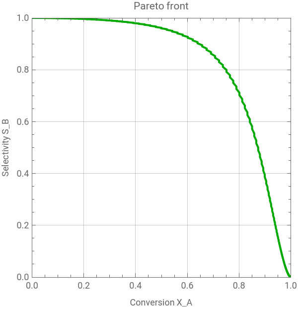
Results (from running the cells above): the grid has 140,800 ( τ ,T) combinations (800 τ values x 176 T values), of which 8,413 -- about 6% -- survive the skyline filter and lie on the Pareto front. The sampled rows of the frontier show the expected monotonic trade-off: at low XA (~0.00004, τ =0.05, T=300 K) selectivity is essentially perfect (SB ~ 0.9999), while at high XA (~0.999, τ ~78.75, T=650 K) selectivity has collapsed to SB ~ 0.00027. Selectivity falls off steeply once XA exceeds roughly 0.6-0.9, which corresponds to the "knee" of the front and is a natural region to look for a balanced operating point.
Visualizing the Trade-off
Visualizing the Trade-off
In[]:=
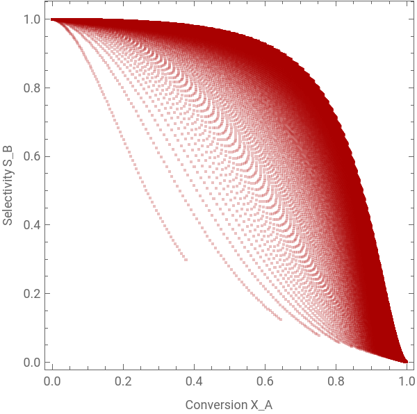
(*Scatter-ploteverygridpoint(dominated+non-dominated)inpalered,*)(*toshowthefullfeasiblecloudinobjectivespace(XA,SB)*)p1=ListPlot[points[[All,{1,2}]],PlotStyle->Directive[Darker@Red,Opacity[0.25],PointSize[0.0006]],PlotLegends->{Style["Dominated designs",Red]},Frame->True,AspectRatio->1,FrameLabel->{"Conversion X_A","Selectivity S_B"},ImageSize->300]
Out[]=

In[]:=
(*Line-plotconnectingtheretained(non-dominated)Pareto-frontpoints*)(*ingreen,andstorethegraphicinp*)p2=ListLinePlot[frontier[[All,{1,2}]],PlotStyle->Directive[Darker[Green],Thick],Joined->True,PlotLegends->{"Pareto front"},PlotLabel->"Pareto front",Frame->True,AspectRatio->1,FrameLabel->{"Conversion X_A","Selectivity S_B"},ImageSize->300,GridLines->Automatic,PlotRange->{{0,1},{0,1}}]
Out[]=

In[]:=
Show[p1,p2]
Out[]=
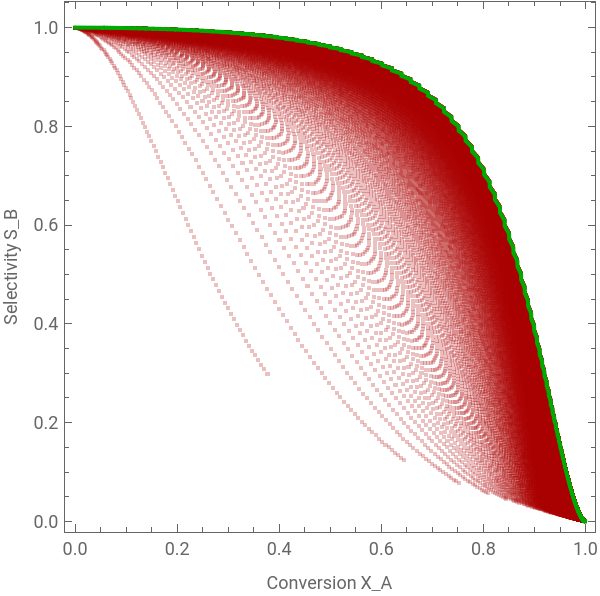
When plotted, allPointsPlot shows the full cloud of 140,800 feasible (XA, SB) designs, and frontierPlot traces its upper-right boundary. The frontier runs from (XA,SB) ~ (0,1) down to ~(1,0): a smooth, concave, monotonically decreasing curve, which is the classic shape for a series reaction A → B → C.
There is no design that improves conversion without cost to selectivity, or vice versa, confirming the two objectives are genuinely in conflict over the whole explored range of τ and T.
There is no design that improves conversion without cost to selectivity, or vice versa, confirming the two objectives are genuinely in conflict over the whole explored range of τ and T.
Selecting a Compromise Design
To pick a single design off the front, we fetch an ideal-point, which minimizes the squared Euclidean distance to the utopia point (XA,SB) = (1,1), i.e. the unattainable design with perfect conversion and perfect selectivity at once.
The minimizer of this distance, subject to the bounds on τ and T, is a natural single "balanced" choice on the Pareto front.
The minimizer of this distance, subject to the bounds on τ and T, is a natural single "balanced" choice on the Pareto front.
Results and Discussion
Running the search above finds sol with minimized squared distance-to-ideal Objective ~ 0.1017 (distance ~ 0.319) at τ ~ 80.02 and T ~ 381.92 K, giving XA ~ 0.737 and SB ~ 0.819 -- i.e. the balanced design converts about 74% of A while retaining about 81% selectivity to B.