Everyone knows about the four seasons of the year since childhood. But as stated in Wiki:
“... a variety of dates and even exact times are used in different countries or regions to mark changes of the calendar seasons. These observances are often declared “official” within their respective areas by the local or national media, even when the weather or climate is contradictory.”
“... a variety of dates and even exact times are used in different countries or regions to mark changes of the calendar seasons. These observances are often declared “official” within their respective areas by the local or national media, even when the weather or climate is contradictory.”
Here I propose an unusual analytical approach to definition of seasons, using computational and visual capabilities of Mathematica (include relatively new powerful TemporalData processing).
Weather data
Weather data
We need minimal and maximal daily temperature in a given geolocation.
Load data
Load data
You can download your custom data and add to dataset. Some values may be missing, so we need to use MissingDataMethod.
This is just example, data are always stored in notebook:
city=;data=TemporalData[WeatherData[city,#,{{firstYear,1,1},{lastYear,12,31},"Day"}]&/@{"MinTemperature","MaxTemperature"},MissingDataMethod{"Interpolation",InterpolationOrder1}];
Geopositions and date samples
Geopositions and date samples
All data required for notebook operation are stored in variable allData , which is initialized at the start.
In[]:=
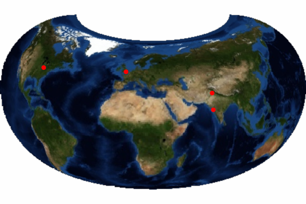
firstYear=2000;lastYear=2010;allData=<|"CLM"<|"loc"->,"minmaxT"|>,"LND"<|"loc"->,"minmaxT"|>,"MMB"<|"loc"->,"minmaxT"|>,"LHR"<|"loc"->,"minmaxT"|>|>;cities=Lookup[Values@allData,"loc"];
GeoGraphics[{Red,PointSize@Medium,Point[cities]},ImageSize->{300,200},GeoRange"World",GeoBackgroundGeoStyling["Satellite"],GeoProjection->"Armadillo",GeoCenter->GeoPosition[{50,25}]]
Extract data
Extract data
In[]:=
Clear[getData];getData[city_,dates_]:=allData[city]["minmaxT"][DateInterval[DateObject[#,"Day"]&/@dates]];
Main idea
Main idea
Let’s select year, find average temperature over this year and plot min-max daily interval with average line for four different geolocations.
In[]:=
year=2006;tmpDatas=getData[#,{{year,1,1},{year,12,31}}]&/@Keys@allData;tMeans=Mean/@tmpDatas;ticks=DateRange[DateObject[{year,1}],DateObject[{year,12}],{1,"Month"}];
It can take 7-8 sec
In[]:=
GraphicsGrid[Partition[MapThread[DateListPlot[#1,Filling{1{2}},GridLines->{Automatic,{{#2,Directive[Thick,Red]}}},FrameTicksStyle->Directive[Bold,10],FrameTicks{{All,All},{ticks,None}},EpilogInset[#3["Name"]<>" "<>ToString[year],Scaled[{.5,.15}]],DateTicksFormat{"MonthNameShort"},ImageSize->{300,150},AspectRatio->1/2]&,{tmpDatas,tMeans,cities}],2]]
Out[]=
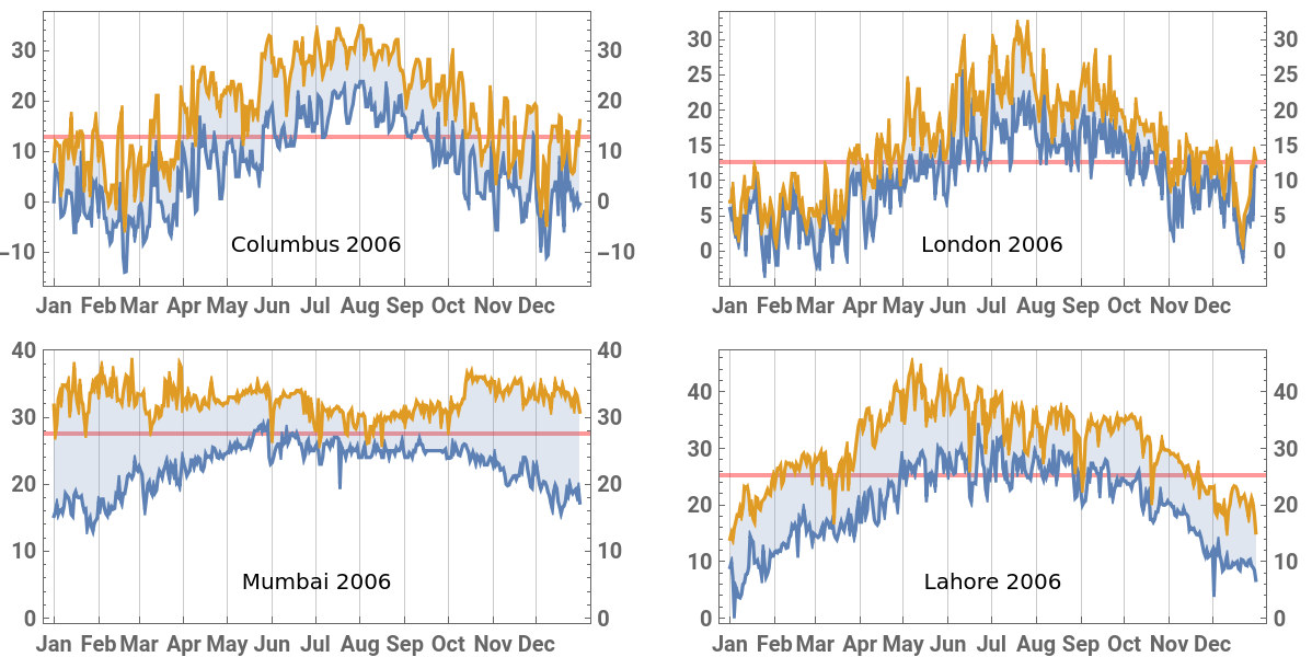
We see that there are days when the daily course of temperature crosses the average. Let’s call them transition days. It can also be observed that there are sufficiently long intervals that do not contain transitional days at all, and intervals consisting entirely of them.
Let us name the periods when the daily temperature does not cross the annual average stable season, and the remaining time - the transition season, and formulate this idea more accurately.
Quantitative formulation
Quantitative formulation
General
General
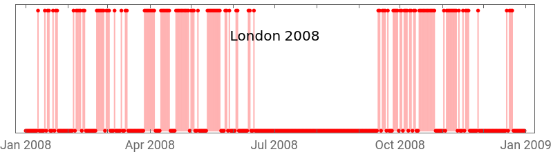
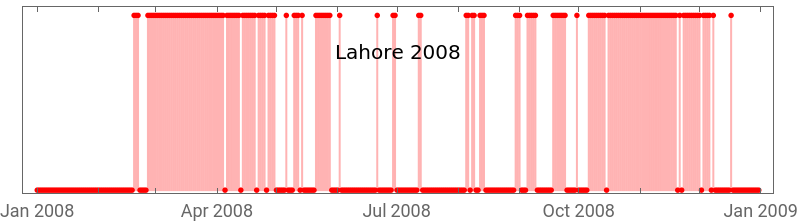
Create boolean TimeSeries with value 1 for transition day and 0 for not
In[]:=
Clear[transDatesBool];transDatesBool[data_]:=With[{tMean=Mean@data},TimeSeriesThread[Boole[First@#<tMean<Last@#]&,data]];
Select two cities and year and look at event-like plots:
In[]:=
generalYear=2008;generalCities={"LND","LHR"};dataRange={{generalYear,1,1},{generalYear,12,31}};generalData=getData[#,dataRange]&/@generalCities;generalTransDays=transDatesBool[#]&/@generalData;Column[MapThread[DateListPlot[#1,FillingAxis,PlotStyle->Red,Joined->False,FrameTicks->{Automatic,None},EpilogInset[allData[#2,"loc"]["Name"]<>" "<>ToString[generalYear],Scaled[{.5,.75}]],ImageSize->400,AspectRatio->1/4]&,{generalTransDays,generalCities}]]
Out[]=
Before we determine seasons, we can make general assessment - the relative number of transition days in the year or seasonality:
In[]:=
Clear[σ];σ[data_]:=1.Total@transDatesBool[data]/data["PathLength"];
Let’s look at plots of this parameter for different years and geolocations. It takes 10-13 secs.
In[]:=
ListLinePlot[Table[σ[getData[c,{{#,1,1},{#,12,31}}]]&/@Range[firstYear,lastYear],{c,Keys@allData}],Mesh->All,DataRange->{firstYear,lastYear},PlotLegends->cities]
Out[]=
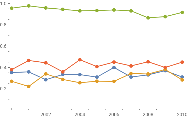


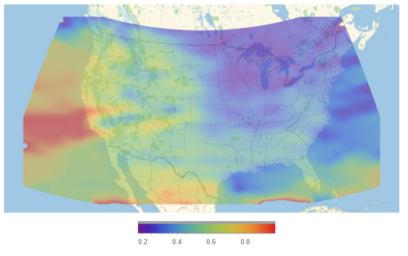
Looks like it’s an indicative characteristic of given location. Here is GeoDensityPlot of the area around USA for many seasonality data, averaged over 10 years.
Seasons detection
Seasons detection
Ideally, there are long continuous periods when all days are either transitional or not.
Then we can distinguish strictly alternating stable (red) and transitional (green) seasons. However, even for geolocations with an apparent seasonality, crossings are uneven. We can try to determine seasons using smoothing filter.
Choose a year and two locations for comparison. Collect data with padding for correct filtering and smooth it with GaussianFilter.
We get a local seasonality factor - the relative number of transition days in the time window containing given date.
With sufficient smoothing we can talk about seasons as periods, when smoothed seasonality lies above or below some selected threshold.
Final example
Final example
Let’s illustrate this idea once again with a separate example. Choose a new geolocation :
This is just example, data are always stored in notebook:
On the basis of smoothing and selection on the threshold find stable and transition seasons (it takes 10-13 sec):
And with Manipulate look at the distribution of stable and transitional seasons in time, taking into account the possible choice of smoothing and the threshold of seasonality:
CITE THIS NOTEBOOK
CITE THIS NOTEBOOK
Detection of yearly seasons in temperature data dependent on average trends and locations
by Denis Ivanov
Wolfram Community, STAFF PICKS, April 23, 2024
https://community.wolfram.com/groups/-/m/t/3163063
by Denis Ivanov
Wolfram Community, STAFF PICKS, April 23, 2024
https://community.wolfram.com/groups/-/m/t/3163063