This project explores how a tunnel diode can push an LC oscillator from equilibrium into more complicated motion. The diode is a quantum device with negative differential resistance, meaning that it can supply energy to the circuit instead of only dissipating it. The notebook starts with the diode’s I-V curve, then develops the circuit equations and studies fixed points and their stability. It then introduces a periodic bias to show period doubling and irregular behavior. Numerical simulations and time-domain waveforms are used to connect the diode’s nonlinear behavior with oscillations in a classical circuit.
Introduction: Quantum tunneling and negative differential resistance
Introduction: Quantum tunneling and negative differential resistance
An LC circuit sets the oscillator’s natural frequency. The tunnel diode changes how the circuit loses and gains energy. In a circuit made only from passive components, the oscillations gradually die out because energy is lost as heat. A tunnel diode can counteract that loss because part of its current-voltage curve has negative differential resistance, or NDR. In this region, the current decreases as the voltage increases. The diode can then supply energy to the circuit instead of only dissipating it, which allows oscillations to continue.
This behavior comes from quantum tunneling. A tunnel diode has a heavily doped p-n junction, which makes its depletion region thin enough for electrons to pass through the barrier. The resulting current-voltage curve has a peak followed by a valley. The section between them is the NDR region. When the circuit’s operating point enters this region, small disturbances can grow instead of dying away. The fixed point becomes unstable, and the circuit can develop a sustained oscillation. In the later driven model, increasing the drive strength changes the shape of the oscillation. The response can move from a simple periodic cycle to period doubling and eventually to chaotic motion.
The tunnel diode I-V model
The tunnel diode I-V model
I model the tunnel diode with a smooth piecewise current-voltage relation . The curve includes the low-voltage turn-on region, the negative differential resistance region, and the forward-conduction branch after the valley point. In the NDR region, <0, so the current decreases as the voltage increases. This negative slope is what allows the diode to supply energy to the oscillator.
I(V)
dI
dV
The calculations use current in amperes, while the plots show current in milliamperes so that the features of the curve are easy to see. To connect the peak and valley, I use a cubic Hermite interpolation. It matches the current values at and , while keeping the slope zero at both endpoints. This lets the curve join the neighboring branches smoothly without a sharp corner.
(,)
V
p
I
p
(,)
V
v
I
v
In[]:=
tdExpr = Piecewise[ { {0, v < 0}, {Ip*(1 - (1 - v/Vp)^3), v <= Vp}, {Ip + (Iv - Ip)* (3*((v - Vp)/(Vv - Vp))^2 - 2*((v - Vp)/(Vv - Vp))^3), v <= Vv} }, Iv + Ifwd*(Exp[alphaF*(v - Vv)] - 1 - alphaF*(v - Vv)) + gForward*(v - Vv)^2 ];dIdVExpr = D[tdExpr, v];tunnelCurrent[x_?NumericQ] := Evaluate[tdExpr /. v -> x];dIdV[x_?NumericQ] := Evaluate[dIdVExpr /. v -> x];
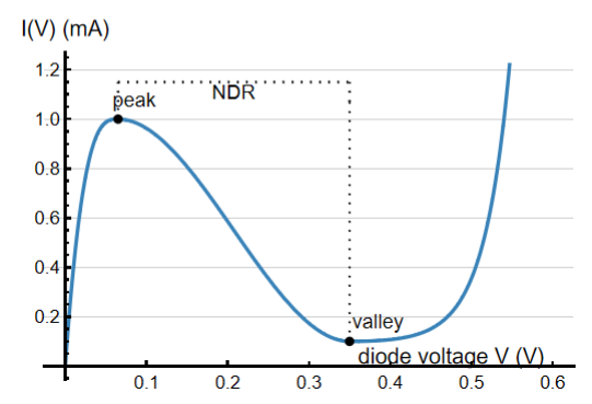
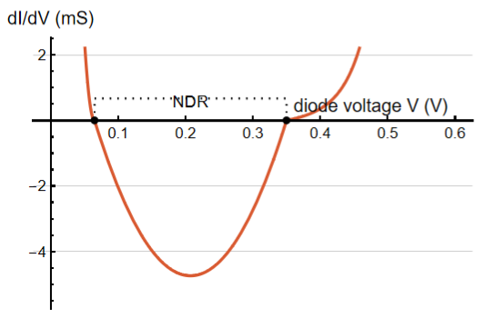
Figure 1: Tunnel diode I-V curve and differential conductance. The black brackets show the negative differential resistance interval, and the right panel shows the conductance crossing zero at the peak and valley points
The left panel shows the tunnel diode’s I-V curve, including its peak and valley. The right panel shows the differential conductance, . The zero line lets us see where the conductance changes sign. Between the peak and valley, is negative, so the diode can supply energy to the circuit instead of only losing it. The code below defines the current law as tdExpr, differentiates it symbolically to get dIdVExpr, and turns both expressions into numerical functions for the circuit simulations that follow.
dI
dV
dI
dV
Circuit equations and fixed point analysis
Circuit equations and fixed point analysis
Kirchhoff’s laws give the circuit equations and A steady operating point is a state where the voltage and current stop changing, so both time derivatives are zero. This gives (), which also means +R(). Here, & describe the fixed point, or the steady state of the circuit.
C-(V)
dV
dt
I
L
I
TD
L-V-R.
d
I
L
dt
V
bias
I
L
*
I
L
I
TD
*
V
V
bias
*
V
I
TD
*
V
*
V
*
I
L
To check whether this state is stable, I use the Jacobian matrix. The Jacobian describes how small changes in voltage and current behave near the fixed point. Its trace is . If a small disturbance dies away, the fixed point is stable. If the disturbance grows, the fixed point becomes unstable. The transition occurs when ()-. At this point, the fixed point loses stability and the circuit can develop a self-sustained oscillation. The tunnel diode supplies energy through its negative differential resistance, which can balance the energy lost in the resistor.
tr(J)-()-
′
I
TD
*
V
C
R
L
′
I
TD
*
V
RC
L
For the parameters used here, the natural frequency of the LC tank is about 0.05 GHz, or 50 MHz. The calculated Hopf bias window is approximately .
{0.07075,0.34975}V
Load line and operating point
Load line and operating point
The load line shows the current that the resistor allows for a chosen bias voltage: -V. The operating point is where this straight line intersects the tunnel-diode I-V curve. At that point, the diode current and resistor current are equal, so the circuit can remain at a steady DC state. If the intersection is outside the NDR interval, small disturbances usually die away. If it moves into the negative-slope region, disturbances can grow and the fixed point can lose stability.
I
L
V
bias
R
In[]:=
L = 1.0*10^-6; (* H *)Ccap = 10.0*10^-12; (* F *)R = 5.0; (* ohm *)findFixedPoint[Vbias_?NumericQ] := Module[{guess, root}, guess = Clip[Vbias, {0.001, 0.58}]; root = FindRoot[ {i == tunnelCurrent[x], Vbias - x - R*i == 0}, {{x, guess}, {i, tunnelCurrent[guess]}} ]; {x, i} /. root ];jacobian[x_?NumericQ] := { {-dIdV[x]/Ccap, 1/Ccap}, {-1/L, -R/L} };criticalSlope = -R*Ccap/L;hopfVoltages = Sort[v /. { FindRoot[dIdVExpr == criticalSlope, {v, Vp + 0.01}], FindRoot[dIdVExpr == criticalSlope, {v, Vv - 0.01}] }];hopfBiases = (# + R*tunnelCurrent[#]) & /@ hopfVoltages;
Out[]=
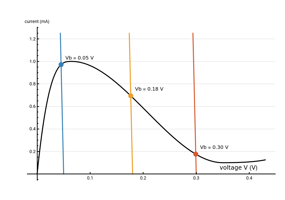
Figure 2: Load-line construction for three bias voltages. The black curve is the tunnel diode I-V characteristic, and the colored lines are the resistor load lines. Their intersections with the diode curve give the circuit’s DC operating points.
In[]:=
circuitSolution[Vbias_?NumericQ, tMax_: 5*10^-7] := Module[{fp}, fp = findFixedPoint[Vbias]; NDSolveValue[ { vc'[time] == (il[time] - tunnelCurrent[vc[time]])/Ccap, il'[time] == (Vbias - vc[time] - R*il[time])/L, vc[0] == fp[[1]] + 1.0*10^-4, il[0] == fp[[2]] }, {vc, il}, {time, 0, tMax}, Method -> "StiffnessSwitching", MaxStepSize -> tMax/5000 ] ]
The black curve is the tunnel diode characteristic, and the three solid colored lines show the resistor load lines for different bias voltages. Each colored point marks the intersection of a load line with the diode curve, so it gives the circuit’s DC operating point. At low bias, the intersection is near the peak of the diode curve. As the bias increases, the operating point moves along the negative-slope section toward the valley, where the fixed point can become unstable and oscillations can begin.
The function findFixedPoint calculates each intersection numerically. The function circuitSolution then uses that fixed point as the initial condition for the time-domain simulation, with a small change to the starting voltage so that any instability can develop.
The function findFixedPoint calculates each intersection numerically. The function circuitSolution then uses that fixed point as the initial condition for the time-domain simulation, with a small change to the starting voltage so that any instability can develop.
Time domain waveforms
Time domain waveforms
The waveforms show the same change over time. At first, the signal repeats in a smooth pattern. As the drive strength increases, the wave becomes distorted and begins alternating between two amplitudes. At higher values, the signal becomes irregular and does not repeat in a simple pattern. This shows how the circuit changes from regular oscillation to chaotic behavior.
Figure 3: Time-domain signatures of the route
Conclusion and Future Directions
Conclusion and Future Directions
A tunnel-diode LC oscillator shows how quantum tunneling can affect the behavior of a classical circuit. The notebook began with the diode’s current-voltage curve, then used load lines and fixed-point analysis to study the circuit’s operating points and stability. The periodically driven model then showed period doubling and chaotic behavior as the drive strength increased. Together, these results show how one nonlinear component can produce different behaviors, from a stable repeating sequence to an irregular sequence. Future work could test more bias and drive values and compare how the oscillation and stability transitions change.
References
References
◼
Cooper, Crystal. “Experimental observation and characterization of chaotic properties in a driven infrared diode circuit.” Chaos, Solitons & Fractals 24.1 (2005): 157-163. https://www.sciencedirect.com/science/article/abs/pii/S0960077904004977
◼
Louodop, Patrick, et al. “Finite-time synchronization of tunnel-diode-based chaotic oscillators.” Physical Review E 89.3 (2014): 032921. https://doi.org/10.1103/PhysRevE.89.032921
◼
Romeira, Bruno, et al. “Synchronisation and chaos in a laser diode driven by a resonant tunnelling diode.” IET optoelectronics 2.6 (2008): 211-215. https://digital-library.theiet.org/doi/abs/10.1049/iet-opt%3A20080024
CITE THIS NOTEBOOK
CITE THIS NOTEBOOK
Quantum tunneling and nonlinear dynamics: from tunnel diodes to chaos
by Guhan Thiagarajan
Wolfram Community, STAFF PICKS, October 12, 2026
https://community.wolfram.com/t/28305
by Guhan Thiagarajan
Wolfram Community, STAFF PICKS, October 12, 2026
https://community.wolfram.com/t/28305