This project presents an Artificial Neural Network (ANN) designed to predict targeted healing perturbations for diseased cellular automata (CAs), effectively restoring and extending their lifetimes. By learning from extensive datasets compromise diseased states of the automaton for a single rule, the model develops a robust understanding of underlying healing mechanisms that transcend specific CA rules. This enables it to generalise healing strategies and suggest effective interventions on previously unseen or untrained CA dynamics and rules, essentially providing treatments for all forms of computational organisms. The ANN bypasses the need for exhaustive explorations of perturbations by directly mapping CA states to therapeutic modifications. In turn this would significantly accelerate recovery prediction in computationally irreducible systems, and inspire remedies for real life scenarios including tissue regeneration, disease therapy, and drug discovery. By uncovering generalised therapeutic patterns, the model provides a framework for developing targetted, data-driven interventions in complex systems characterized computationally irreducible behaviors.
Introduction
Introduction
In the search for a formal computational foundation for medicine, one central challenge emerges: how can we mathematically represent “disease” and then learn how to reverse it? In this computational essay, I explore a conceptual model model that treats disease as a perturbation in a digital organism, represented by a cellular automaton, and attempts to “heal” it using a neural network trained to apply corrective interventions.
Inspired by Stephen Wolfram’s work on the computational formalization of medical systems, this project operates at the intersection of machine learning and pathology. The cellular automaton is treated as a simplified computational organism whose evolution reflects its internal “health.” A deviation from expected patterns (such as an early death or chaotic decay) constitutes a pathological state, akin to a disease in biological systems.
The central idea is to develop a model that, when given a diseased version of a cellular automaton, can learn to predict a targeted perturbation - an intervention - which returns the system to a healthier or longer-living state. In essence, we attempt to compute the therapeutic logic behind medical treatments by not merely detecting what’s wrong, but suggesting what should be done to fix it.
Cellular Automata as Computational Organisms
Cellular Automata as Computational Organisms
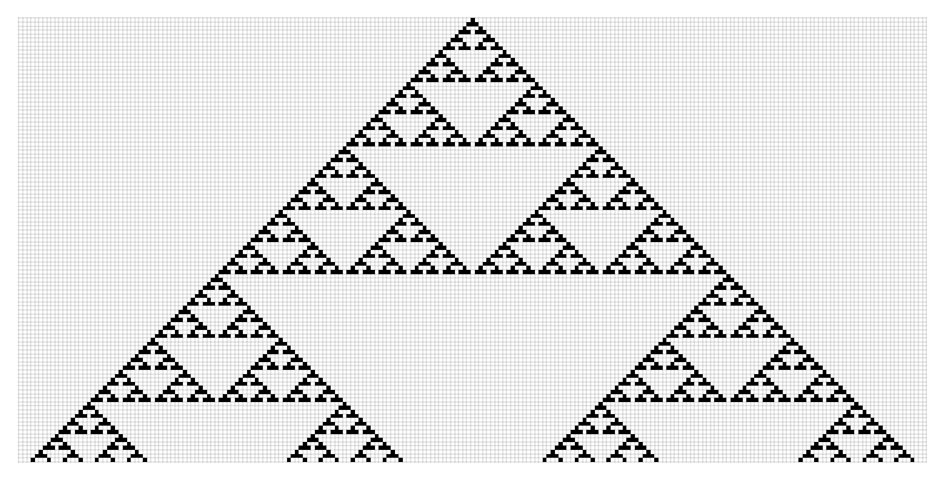
Cellular automata (CA) are idealized, rule-based systems composed of discrete cells evolving over time. Despite their simplicity, they are capable of generating complex behaviors that mimic lifelike dynamics including growth, symmetry, differentiation, and decay. Below is an example of a simple cellular automata, with the value 1 being represented by Black, and value 0 being represented by White. The rules of the automaton applies is also shown.
Row[{ArrayPlot[ArrayPad[CellularAutomaton[22,{{1},0},110],{{0,0},{3,3}}],ColorRules{0White,1Black},ImageSize{Automatic,520},MeshAll,MeshStyleOpacity[0.1`]],(GraphicsGrid[#1,DividersDirective[Thin,GrayLevel[0.6`]],ImageSize280]&)[(Partition[#1,UpTo[8]]&)[Flatten[RulePlot[CellularAutomaton[22],ColorRules{0White,1Black}]〚1,1,All,All,1〛]]]},Spacer[20]]
Out[]=


Similarly, we can apply different rules of the automaton, to get different shapes. In this model, we consider a cellular automaton initialized with a specific state (the “birth” of the organism). Under a given rule, it evolves generation by generation. Typically, a healthy automaton lives for many steps with its active, non-zero states persisting through time. Shown below is one such “organism” made from cellular automata.
Out[]=
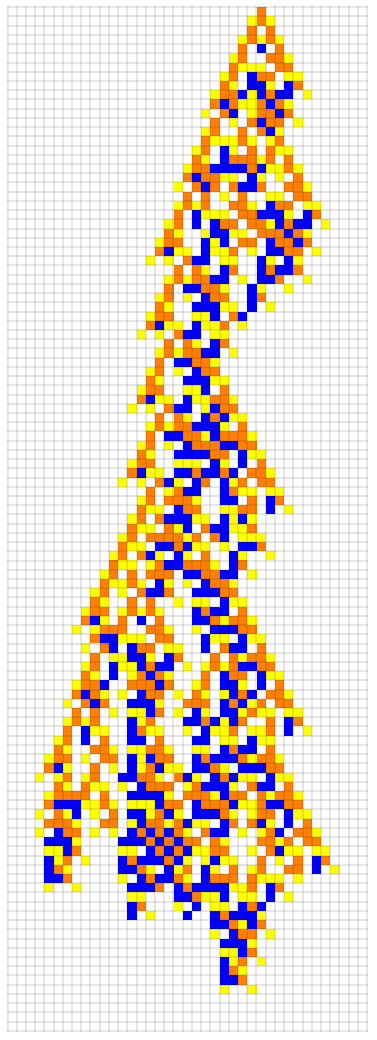
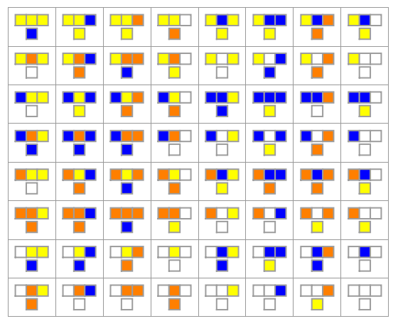
Additionally, the rules of the organism - acting somewhat like its “genetic code” is also shown. Here the “organism” or any cellular automata is being progressively constructed by repeatedly applying the rules on the right side. Looking at our model in detail, it can be seen that it is a grid of squares, each having one of 4 possible colors (white, orange, blue, yellow). The rules here are very simple, but we can see that when we run the rules, it leads to a complicated pattern. This pattern “dies out” (all cells become white) after exactly 107 steps, known as the lifetime of the organism. Therefore, the healthy/natural lifetime of this organism is 107, meaning it survives for 107 steps before “dying” out (all cells are white).
In this model, we go beyond the conventional binary cellular automaton, where each cell is either 0 or 1. Instead, we extend the system to a quaternary-state cellular automaton, where each cell can take on one of four discrete states: 0, 1, 2, or 3. This increased state space allows for a richer variety of local interactions and global behaviors, mimicking the increased complexity of biological organisms where individual components (such as cells or molecules) exist in multiple functional states rather than being simply “on” or “off.” The additional states introduce more diverse pattern formation, symmetry-breaking behaviors, and failure modes, making the automaton a more representative computational analogy of a living system.
In this system, the state 0 is visually represented as white, symbolizing the absence of activity or the “death” of the cellular automaton. When all cells in the grid transition to state 0, it indicates that the organism has ceased functioning, its lifetime has ended. The other possible cell states (1, 2, and 3) are assigned distinct colors, selected arbitrarily for visualization purposes, to differentiate the active regions of the organism. These color assignments have no computational significance but provide an intuitive way to observe how the organism develops, decays, and responds to perturbations over time.
What are Perturbations?
What are Perturbations?
In biological systems, illness is rarely the result of randomness; rather, it often stems from some external or internal disturbance – whether it be a genetic mutation, an infection, or physical trauma. Translating this concept to our computational setting, we define disease in cellular automata as a deviation from normal behavior caused by an external modification to the system’s initial state. These modifications, known as perturbations (or computational “insults”), disrupt the automaton’s natural evolution and introduce pathological dynamics.
Within our model, a perturbation refers to an intentional change applied to one or more cells at the very beginning of the automaton’s life. In its untouched form, the cellular automaton follows a predictable rule set, evolving smoothly from its initial seed. But once a perturbation is introduced, even a single altered cell changes how the rule propagates through the system, cascading into vastly different long-term behavior. What would have been a stable, healthy organism with a lifespan of 107 steps might now decay prematurely – collapsing in just some 50 steps. Alternatively, in some rare cases, the system adapts to the disturbance, stabilizing into a longer-lived form, illustrating a kind of computational resilience or self-healing.
Within our model, a perturbation refers to an intentional change applied to one or more cells at the very beginning of the automaton’s life. In its untouched form, the cellular automaton follows a predictable rule set, evolving smoothly from its initial seed. But once a perturbation is introduced, even a single altered cell changes how the rule propagates through the system, cascading into vastly different long-term behavior. What would have been a stable, healthy organism with a lifespan of 107 steps might now decay prematurely – collapsing in just some 50 steps. Alternatively, in some rare cases, the system adapts to the disturbance, stabilizing into a longer-lived form, illustrating a kind of computational resilience or self-healing.
Here we generate the “healthy” cellular automaton. The long weird looking number is the rule for this particular cellular automata. And I used array plot to graph it.
healthyCellularAutomaton=ArrayPlot[CellularAutomaton[{252507139021300249072588345221334974732,4,1},{{1},0},{150,{-100,100}}],PlotLabel->"Healthy",ColorRules->{0->White,1->Orange,2->Blue,3->Yellow}];
In[]:=
pertubedCellularAutomaton=Module[{ca=First[#],pert=Last[#]},ArrayPlot[ca,PlotLabel->"Diseased Automaton",ColorRules->{0->White,1->Orange,2->Blue,3->Yellow},Epilog->{Red,Arrowheads[Medium],Arrow[{{-100,Length[ca]-#1+.5},{#2-.5,Length[ca]-#1+.5}}]&@@@Keys[pert]}]]&[ResourceFunction["PerturbedCellularAutomaton",ResourceSystemBase->"https://www.wolframcloud.com/obj/resourcesystem/api/1.0"][{252507139021300249072588345221334974732,4,1},{{1},0},{150,{-100,100}},{{9,96}->1}]];
In[]:=
selfHealedCellularAutomaton=Module[{ca=First[#],pert=Last[#]},ArrayPlot[ca,PlotLabel->"Self-Healing Automaton",ColorRules->{0->White,1->Orange,2->Blue,3->Yellow},Epilog->{Red,Arrowheads[Medium],Arrow[{{-100,Length[ca]-#1+.5},{#2-.5,Length[ca]-#1+.5}}]&@@@Keys[pert]}]]&[ResourceFunction["PerturbedCellularAutomaton",ResourceSystemBase->"https://www.wolframcloud.com/obj/resourcesystem/api/1.0"][{252507139021300249072588345221334974732,4,1},{{1},0},{150,{-100,100}},{{23,103}->3}]];
GraphicsRow[{healthyCellularAutomaton,pertubedCellularAutomaton,selfHealedCellularAutomaton},ImageSize->Full]
Out[]=
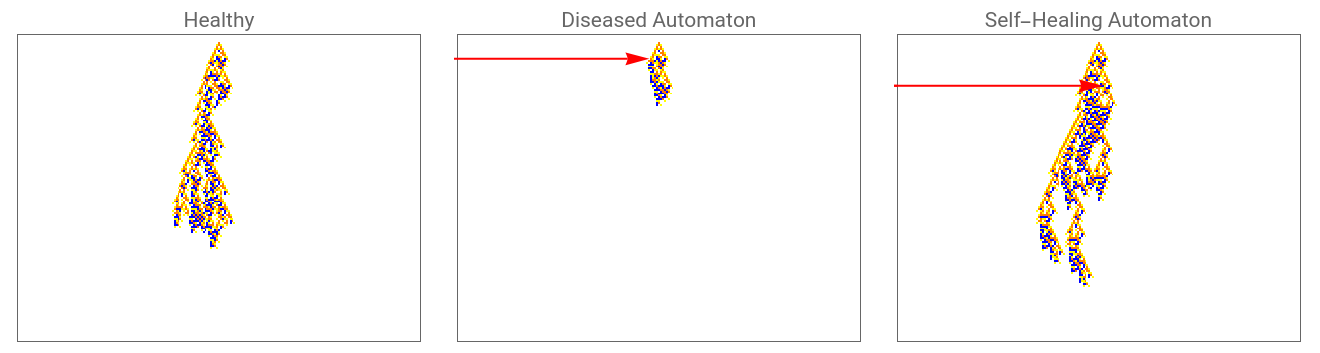
The arrow in the diagram highlights a single cell within the automaton that has been perturbed, meaning that its state has changed from what the original cellular automaton would have produced. This small modification at an early stage might seem insignificant in isolation, yet when the system evolves over time, the effects can be profound. In some cases, this perturbation causes the automaton to “die” much sooner than expected, its active body disappearing prematurely. But intriguingly, in other cases, the perturbation actually increases the automaton’s lifetime, effectively allowing it to self-heal, compensating for the disturbance and even extending its existence beyond the unperturbed, “healthy” baseline. This is the computational equivalent of resilience (the system adapts and stabilizes in the face of disruption).
In this context, perturbations represent the computational abstraction of medical pathology. Just as in biological systems, where diseases arise from genetic mutations, environmental stresses, or pathogen invasions, perturbations introduce disturbances that alter the normal functioning of our digital organism. By applying these perturbations systematically and observing their consequences, we are in effect modelling the disease landscape of our artificial life forms. Some perturbations are benign, causing little or no harm. Others are devastating, fundamentally disrupting the automaton’s ability to sustain its structure and processes.
One of the most fascinating phenomena revealed through these experiments is how sensitive and unpredictable these computationally-defined systems can be. A minor change in the state of a single cell may dissipate harmlessly within a few steps, while a seemingly identical perturbation in another location or with a slightly different value might cascade through the system, dramatically shortening – or lengthening – the organism’s lifetime. This mirrors a key challenge in real-world medicine: the same mutation, viral infection, or therapeutic intervention can have radically different effects depending on the broader biological context. Predicting outcomes from first principles becomes infeasible in such complex systems.
However, unlike living biological systems – where experimentation is constrained by ethical concerns, time, and cost – cellular automata provide a computational sandbox where we can run thousands of experiments in rapid succession. Each perturbation, lifetime measurement, and emergent pattern contributes to a growing body of computational data. This process allows us to explore the space of possible diseases and recoveries far more exhaustively than would ever be feasible in traditional biology.
This computational exploration of pathology and healing not only gives us insight into the behavior of complex systems but also provides the rich dataset we need for the next stage of the project: training a model to learn from these perturbations and suggest new interventions that promote healing. In other words, this system becomes a virtual laboratory – an environment where computational experiments accelerate the search for interventions, helping us understand how to restore balance to diseased systems, whether they be artificial organisms or, someday, biological ones.
Discovering Computational Healing
Discovering Computational Healing
The ultimate aim of this project is to predict the therapeutic perturbation needed for a diseased digital organism, represented as an insulted CA, to actively intervene and restore the behavior toward its healthy state. While previous works have analyzed the biological evolution CA as dying off after a certain number of steps, this approach delves deeper into discovering a second perturbation needed to extend the lifetime. The question is not just “What is wrong with this organism?” but “What can we do to fix it?”
But finding such a healing perturbation is far from straightforward. While the rules governing the organism are explicitly defined, the way perturbations interact with those rules over time is computationally complex and irreducible: the only way to know whether a perturbation works is to try it and observe the outcome. Analytical shortcuts fail, and the combinatorial explosion of possible perturbations makes brute-force search impractical . This leads us to a fundamental challenge.
But finding such a healing perturbation is far from straightforward. While the rules governing the organism are explicitly defined, the way perturbations interact with those rules over time is computationally complex and irreducible: the only way to know whether a perturbation works is to try it and observe the outcome. Analytical shortcuts fail, and the combinatorial explosion of possible perturbations makes brute-force search impractical . This leads us to a fundamental challenge.
In[]:=
healthyCa1=ArrayPlot[CellularAutomaton[{252507139021300249072588345221334974732,4,1},{{1},0},{150,{-100,100}}],ColorRules->{0->White,1->Orange,2->Blue,3->Yellow},PlotLabel->"Healthy Automaton"];
In[]:=
perturbedCa1=Module[{ca=First[#],pert=Last[#]},ArrayPlot[ca,PlotLabel->"Diseased Automaton",ColorRules->{0->White,1->Orange,2->Blue,3->Yellow},Epilog->{Red,Arrowheads[Medium],Arrow[{{-100,Length[ca]-#1+.5},{#2-.5,Length[ca]-#1+.5}}]&@@@Keys[pert]}]]&[ResourceFunction["PerturbedCellularAutomaton",ResourceSystemBase->"https://www.wolframcloud.com/obj/resourcesystem/api/1.0"][{252507139021300249072588345221334974732,4,1},{{1},0},{150,{-100,100}},{{41,91}->3}]];
In[]:=
healedCa1=Module[{ca=First[#],pert=Last[#],coords},coords=Keys[pert];ArrayPlot[ca,PlotLabel->"Healed Automaton",ColorRules->{0->White,1->Orange,2->Blue,3->Yellow},Epilog->{{Red,Arrowheads[Medium],Arrow[{{-100,Length[ca]-coords[[1,1]]+0.5},{coords[[1,2]]-0.5,Length[ca]-coords[[1,1]]+0.5}}]},{Black,Arrowheads[Medium],Arrow[{{-100,Length[ca]-coords[[2,1]]+0.5},{coords[[2,2]]-0.5,Length[ca]-coords[[2,1]]+0.5}}]}}]]&[ResourceFunction["PerturbedCellularAutomaton",ResourceSystemBase->"https://www.wolframcloud.com/obj/resourcesystem/api/1.0"][{252507139021300249072588345221334974732,4,1},{{1},0},{150,{-100,100}},{{41,91}->3,{51,92}->0}]];
This code visualizes a healed cellular automaton after applying specific perturbations. It first extracts the cellular automaton grid (ca) and the perturbations (pert). The coordinates of the perturbations are identified and used to annotate the plot. ArrayPlot is used to display the automaton, with a custom color scheme where each cell value (0 to 3) corresponds to a specific color. Two arrows are drawn on the plot using Epilog, pointing from the left side of the plot to the locations of the two perturbations: one red arrow and one black arrow, indicating where the healing modifications were applied. The automaton data is generated by evolving a perturbed cellular automaton using a specified rule and initial conditions through a Wolfram resource function.
GraphicsRow[{healthyCa1,perturbedCa1,healedCa1},ImageSize->Full]
Out[]=
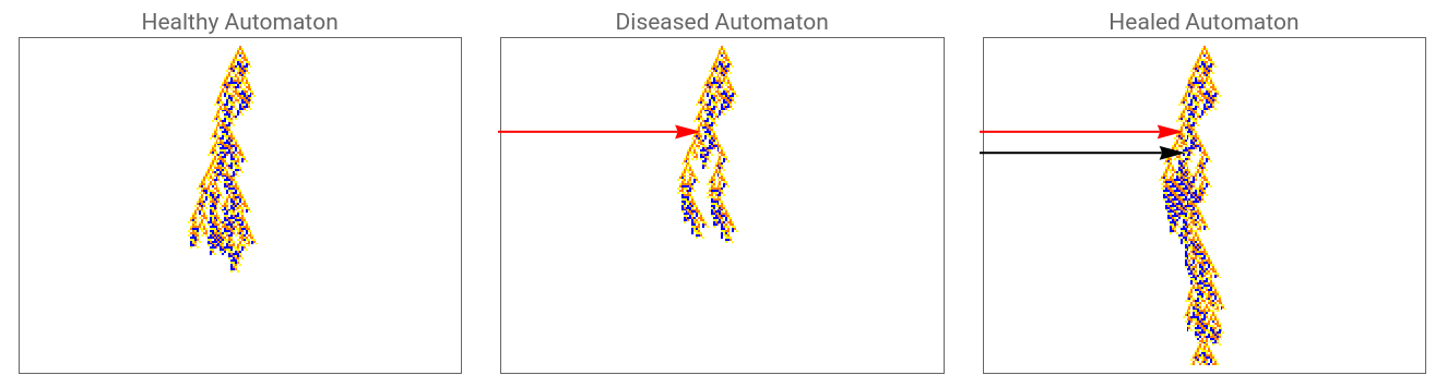
Here, the red arrow shows the initial perturbation that was applied to the healthy CA, which caused it to be diseased. The black arrow then shows the additional “therapeutic” perturbation that was made, which increased the lifetime of the automaton.
Width History
Width History
Width history refers to the temporal sequence of the active region’s size or spatial extent in a cellular automaton over successive time steps. Specifically, it tracks the number of cells in the CA that are in a non-quiescent (active) state at each iteration, effectively capturing how the pattern grows, shrinks, or stabilizes as the automaton evolves. This one-dimensional time series provides a concise summary of the CA’s dynamic behavior and is useful for analyzing its overall activity and health, as changes in width can indicate progression or regression of “disease” within the system. Essentially, the width history is the raw CA data.
Mitigating the Challenges of Computational Irreducibility
Mitigating the Challenges of Computational Irreducibility
In a computationally irreducible system, the only way to determine the outcome after a certain number of steps is to explicitly simulate the system step by step. There is no shortcut formula, no closed-form solution that can predict the future state without performing the actual computations. Essentially, as illustrated below, the only way to know how an organism will evolve is to run the simulation and watch what happens.
ArrayPlot[CellularAutomaton[CellularAutomaton[30],{{1},0},50],ImageSize->Large]
Cellular automata are classic examples of such systems (simple one shown above). Despite having simple underlying rules, they generate highly complex and unpredictable behavior over time. Even a single-cell perturbation in the initial state can cascade into drastically different long-term patterns. As a result, we cannot analytically determine how a disease-like perturbation affects the lifetime of the organism, nor can we “reverse engineer” a diseased system back to its healthy origin using a deterministic algorithm.
Instead, we must explore the space of possible perturbations experimentally, systematically applying them and observing their effects on the automaton’s lifetime. But this search space is vast, with hundreds of potential body cells and three possible values for each (0-3 other than the current value), the number of possible perturbations grows exponentially. Exhaustively testing all combinations is computationally impractical.
This is where neural networks come in. Neural networks do not attempt to directly solve the irreducible dynamics of the cellular automaton. Instead, they operate as pattern recognizers, learning correlations between observable symptoms (the current diseased CA pattern and its lifetime) and effective healing interventions, based on the outcomes of prior simulations. Neural networks don’t bypass or solve computational irreducibility, instead they offer a way to learn useful heuristics and approximations within it. They effectively identify statistical regularities – small computational shortcuts – that can guide us toward more promising perturbations without needing to simulating every possibility.
Generation of Diseased Cellular Automatons
Generation of Diseased Cellular Automatons
Creating a function to generate a diseased cellular automaton for a given rule, as it is needed in succeeding functions:
This function was created to generate diseased Cellular Automatons fast. Since the original lifetime of the organism is 107, “diseased” is defined as perturbed automatons with lifetime less than 107. This function helps in data collection where multiple diseased automatons were required. The third item in the list shows the lifetime of the CA generated by the function; as expected, since it is less than 107, it is diseased.
Data Collection With Perturbation Testing
Data Collection With Perturbation Testing
One of the most important, and admittedly one of the most computationally intensive, parts of this project was the perturbation testing function. Essentially, it takes a diseased cellular automaton, then tries perturbations on its body coordinates, and checks the effects of the perturbation on the lifetime of the automaton. The reason why it is so computationally intensive is perturbing dozens or hundreds of active cells, and multiple possible values (0 to 3) for each perturbation, the number of possible perturbations is huge. This is why we need a systematic way to try them all efficiently and record which ones lead to better outcomes.
Without this process, we would have no data to teach a neural network. The neural network learns from examples of what worked and what didn’t work, exactly the kind of data this function produces.
Without this process, we would have no data to teach a neural network. The neural network learns from examples of what worked and what didn’t work, exactly the kind of data this function produces.
Creating a function which tests all body coordinates of the diseased CA for all 4 values (other than its current value) and appending the results:
Since cellular automata are computationally irreducible, we can’t look at the grid or apply a formula to figure out which perturbation would heal the system. The only way to know that is to apply it, evolve the system, and measure the lifetime again.
The function takes in a diseased automaton, along with initial perturbation that was applied before. It then calculates the baseline lifetime of the diseased automaton, being the starting point for comparison. It then finds all the body coordinates (active cells) of the organism, where a perturbation might have some effect, as perturbing empty space would be inefficient and redundant. For each active cell, the function replaces its state with each possible value (0, 1, 2, 3), except for the cell’s current state value.
After that, each perturbation is recorded. It also records the coordinate where it was applied, the new value that was tested, and information about the new lifetime—its improvement and “health” range. Finally, the function filters in only the perturbations that produced a lifetime improvement, sorted by their improvement level, and identifies the best perturbation found.
Test All Perturbations Visualization
Test All Perturbations Visualization
This was one of the most important functions for data collection, which is why it is important to fully understand what exactly is happening in this function. Which can be seen in the animation below:
Generating diseased CA and setting a fixed value:
This code generates a diseased cellular automaton. To focus on the active regions of the CA, the function bodyCoordinates is used to obtain a list of coordinates corresponding to the CA’s body cells, which is saved as bodyCoordsForAnimation. Finally, a fixed value of 1 is assigned to fixedValue, meaning that for each coordinates the value will be changed to 1.
This function visualizes a perturbed cellular automaton by applying a fixed perturbation at a given coordinate and overlaying an arrow to clearly indicate the location of the intervention:
This code defines a function perturbedCAWithArrow that visualizes a cellular automaton (CA) with a highlighted perturbation at a specific coordinate. The function takes the CA grid and a coordinate coord as inputs. It creates a new CA state by replacing the cell at coord with a fixed value (1). An arrow is drawn on the plot pointing to the perturbed cell location, using coordinate transformations to correctly position it on the displayed grid. The CA is visualized with ArrayPlot, applying specific colors for each cell state and overlaying the red arrow and a label indicating the perturbed coordinate and value.
the code generates a list of frames by applying perturbedCAWithArrow to each coordinate in bodyCoordsForAnimation, creating a sequence of visualizations showing the perturbation moving through all active cells. Finally, ListAnimate displays these frames as an animation lasting 15 seconds, providing an intuitive, dynamic view of the perturbation process across the CA body.
The process shown above is only for one diseased cellular automaton, and it is only changing it to 1 value.
While this process is a bit computationally intensive and we are essentially finding brute forced solutions , it is critical because it gives us ground truth data. For any diseased CA, we now know exactly which perturbations helped it recover, and which ones didn’t, which is useful for the training data for the neural network. And after training of the neural network, it would allow us to approximate the “growth” of the CA, requiring lower computations.
While this process is a bit computationally intensive and we are essentially finding brute forced solutions , it is critical because it gives us ground truth data. For any diseased CA, we now know exactly which perturbations helped it recover, and which ones didn’t, which is useful for the training data for the neural network. And after training of the neural network, it would allow us to approximate the “growth” of the CA, requiring lower computations.
Model Training
Model Training
we are shifting the target values of the perturbation from a 0-based to a 1-based index. This adjustment is important because Softmax expect class labels to start from 1, not 0.
In our problem, the original perturbation values range from 0 to 3, representing the possible cell states in the cellular automaton. However, when training the neural network’s classification output, we need the target labels to be 1, 2, 3, 4, to align with the softmax output’s class indices.
Mathematically, if the original target space is:
V = {0, 1, 2, 3}
we shift it to:
V’ = {1, 2, 3, 4}
so that each class index corresponds correctly to a neuron in the softmax layer’s output vector.
This is a simple mapping, but it ensures Softmax correctly interprets the labels during training.
This is a simple mapping, but it ensures Softmax correctly interprets the labels during training.
Creating a training dataset by pairing each input with its corresponding coordinate regression target and categorical value target:
We reshape the training data and explicitly label its components because neural networks require input and output data to be structured in a form that matches the architecture of the network. To make sure each part of the network receives the correct target during training, we explicitly construct each data sample as an association containing three parts: the “Input” field (the flattened body mask of the CA), “Output1” (the 2D coordinate target for the regression branch), and “Output2” (the class label for the classification branch).
This labeling not only clarifies which output corresponds to which branch of the neural network, it also ensures that the training process applies the appropriate loss functions and shape validations for each output type. For instance, “Output1” must match the shape and type expected by the coordinate regression layer, while “Output2” must match the class indices expected by the softmax classification layer. Without this structure, the neural network would be unable to correctly align its predictions with the ground truth, leading to errors during training or inaccurate learning. Thus, by reshaping and clearly labeling the data, we create a training dataset that efficiently interfaces with the computational framework of the neural network, enabling it to learn both continuous spatial predictions and discrete perturbation values in a single, unified training process.
This labeling not only clarifies which output corresponds to which branch of the neural network, it also ensures that the training process applies the appropriate loss functions and shape validations for each output type. For instance, “Output1” must match the shape and type expected by the coordinate regression layer, while “Output2” must match the class indices expected by the softmax classification layer. Without this structure, the neural network would be unable to correctly align its predictions with the ground truth, leading to errors during training or inaccurate learning. Thus, by reshaping and clearly labeling the data, we create a training dataset that efficiently interfaces with the computational framework of the neural network, enabling it to learn both continuous spatial predictions and discrete perturbation values in a single, unified training process.
Training the Neural Network Based on the Width History Training Data:
Training Plots
Training Plots
Coordinate (Output1) Loss
Coordinate (Output1) Loss
This plot shows the loss curve for the regression task, where the neural network predicts the coordinate (x, y) of the perturbation. The vertical axis is on a logarithmic scale, showing how the loss starts off relatively high and decreases consistently over time. The smooth downward trend suggests that the model is progressively minimizing the difference between its predicted coordinates and the actual target coordinates from the training data. Although some noise is visible, the general trajectory reflects effective learning. This regression task is harder to optimize, since coordinates are continuous values and errors are measured precisely, so a slower convergence is expected compared to the classification task.
Value (Output2) Loss
Value (Output2) Loss
For Output 2, which corresponds to the classification of the perturbation value, the second plot shows the cross-entropy loss, which is a standard metric for multi-class classification tasks. The vertical axis is on a logarithmic scale, so a value of 1 corresponds to relatively high uncertainty in the model’s predictions. As training progresses, the loss steadily drops below 1, indicating that the model is becoming more confident and accurate in predicting the correct perturbation value class (0, 1, 2, or 3).
A cross-entropy loss below 1 for a 4-class problem suggests that the network is moving significantly beyond random guessing (which would give a cross-entropy loss close to ln(4) ≈ 1.39). This shows that the network is successfully learning meaningful patterns in the body structure that correlate with the correct healing perturbation values. While some fluctuations remain due to the complexity of the problem and data variability, the overall downward trend reflects steady optimization.
A cross-entropy loss below 1 for a 4-class problem suggests that the network is moving significantly beyond random guessing (which would give a cross-entropy loss close to ln(4) ≈ 1.39). This shows that the network is successfully learning meaningful patterns in the body structure that correlate with the correct healing perturbation values. While some fluctuations remain due to the complexity of the problem and data variability, the overall downward trend reflects steady optimization.
Error Rate
Error Rate
This plot shows the error rate for the classification task (predicting the perturbation value) over successive training rounds. Initially, the error rate is very high, close to 75%, which is expected in a multi-class classification task where the model begins without any understanding of the task. Over time, as the network learns from more examples, the error rate steadily decreases. By the 50th round, the error rate has dropped below 25%, showing that the network has learned useful patterns from the data. This decrease suggests that the network is successfully identifying the correlation between body structures and the correct perturbation values. Some oscillations remain due to the stochastic nature of training and possibly the limited dataset size or variability in the CA patterns.
Model Testing
Model Testing
This line adjusts the values to be greater than 0 for the softmax function:
This line applies the trained neural network (trainedNetExample) to each test input in testInputs, storing the output predictions in the list testPredictions. Each prediction is assumed to be an association containing multiple outputs:
This line applies the trained neural network to each test input in testInputs, storing the output predictions in the list testPredictions. Each prediction is assumed to be an association containing multiple outputs:
This selects the most probable value for the value out of 0,1,2,3:
This calculates the Euclidean distance between each predicted coordinate and the true target coordinate, resulting in a list of coordinate errors:
This produces a list of booleans indicating whether the predicted perturbation value matches the true target value for each test sample:
Computes the average Euclidean distance error and accuracy over all test samples:
The above shows the accuracies and errors for the model trained on 10 diseased automatons.
To further improve the accuracy of the model, I trained the original model on 1000 diseased automatons, which was a very tedious process; So below, I am importing the trained model on 1000 diseased CA’s. This model was tested on 200 diseased automatons (0.2*100), with a value accuracy of 0.66, and Euclidean Distance of 7.7.
Imports the trained neural network:
The NetTrain function is used to optimize the parameters of the network. We explicitly define two distinct loss functions, one for each output branch of the model, aligning with the dual-task nature of the problem:
For “Output1”, corresponding to the coordinate regression, we use Mean Squared Loss, a standard loss for regression tasks that penalizes deviations between predicted and actual coordinates.
For “Output2”, which predicts the perturbation value class, we use Cross Entropy Loss with class indices, which is the conventional choice for classification problems with discrete target categories.
This dual-loss formulation allows the network to independently learn both continuous-valued spatial predictions and discrete perturbation classifications. The network optimizes both losses simultaneously during backpropagation, balancing the accuracy of spatial targeting with the correctness of perturbation values.
We specify a BatchSize of 8, meaning that in each training iteration, the network processes 8 samples in parallel. This is a trade-off between computational efficiency and convergence stability. Smaller batch sizes make training noisier but allow for faster updates and better generalization in some cases. A MaxTrainingRounds of 50 controls the total number of full passes through the training dataset, ensuring the model does not overfit or underfit.
In essence, this block efficiently initiates the parameter optimization loop, iteratively adjusting the neural network’s weights to minimize the combined regression and classification loss, thus learning to predict effective healing perturbations for diseased cellular automata.
Prediction Function
Prediction Function
To make the process of obtaining predictions from the model easier, we are creating a function for it.
Creating the prediction function which takes the width history as an input and output the predicted coordinate and value:
This function processes a raw CA by creating a binary mask of active cells, flattens it, and feeds it into the trained neural network. It then extracts the predicted perturbation coordinates and value probabilities, selects the most likely value, and clamps the coordinates within the CA bounds. The result is returned as an association with the predicted coordinate and perturbation value.
Visual Results From the model
Visual Results From the model
Here we get the first diseased CA (The coordinate is specified because the resource function randomizes the coordinate when coordinate is not specified):
We got the model prediction from the initially perturbed automaton:
Applying the perturbation generated by the model:
This result shows a dramatic recovery of the cellular automaton’s lifetime: the organism originally survived for only 31 steps in its diseased state, but after applying the predicted healing perturbation, it recovered to 149 steps, almost its maximum potential. This is not a minor adjustment, but a near-complete restoration of its healthy lifespan. The cellular automaton, which at first glance appeared irreversibly damaged, was able to regenerate its dynamics and sustain itself far longer than before, purely through an intelligently chosen, data-driven perturbation.
This outcome illustrates the deeper success of this work. Despite the computational irreducibility of the system – where no shortcuts exist to directly calculate the future behavior of the automaton – the neural network was able to find effective interventions. It did not “solve” computational irreducibility in the strict sense, but it navigated around it, learning empirical correlations that humans would never find by hand, and predicting interventions that extend the organism’s lifespan without requiring full analytical understanding of its inner workings.
This is what makes the project so exciting. It demonstrates that, in complex dynamical systems where traditional mathematical modeling fails, machine learning models can still learn useful intervention strategies. This opens up applications far beyond cellular automata. The same approach could be applied to synthetic biology, drug discovery, and genetic engineering, where the underlying systems are too complex to model exactly, but where data-driven experimentation can reveal life-extending or disease-reversing interventions. It suggests a future where we use neural networks not only to predict outcomes but to design healing actions in systems as complicated and unpredictable as life itself.
Above the lifetime of the diseased cellular automaton increased from 41 to 147, which is a increase of 106 in the lifetime of the automaton.
Above is another example showing the massive increase in lifetime in lifetime due to the coordinates predicted by the model.
Rule-generalization capability
Rule-generalization capability
One of the fundamental challenges in studying cellular automata is that even small changes in the underlying rule can completely alter the system’s dynamics. Each rule defines a unique computational universe, with its own evolutionary behaviors and sensitivities to perturbation. Therefore, a natural question arises: Does the trained neural network, which has learned healing perturbations for one specific rule, generalize to other rules, or is its learning strictly rule-dependent?
In this section, we investigate the rule-generalization capability of our model. Cellular automata, by their nature, exist in a vast design space of rules – each defining a different computational irreducible system. While our model has been trained on data generated from a fixed rule, its input features are not the raw CA evolution itself, but the encoded structure of the organism’s body. This suggests the possibility that the neural network has learned structural healing patterns, rather than rule-specific shortcuts.
By applying the trained model to cellular automata governed by new, unseen rules, we test whether the model’s learned representations are robust across computational systems, or whether its understanding of healing is fundamentally tied to the dynamics of the rule it was trained on.
It can be clearly observed that the model predicted an effective therapeutic perturbation on a cellular automaton governed by a completely different ruleset—one that it had never encountered during training. Remarkably, despite the altered computational dynamics, the model was still able to localize a meaningful intervention, resulting in a substantial lifetime improvement of 31 steps. This outcome demonstrates a level of generalization beyond what one might expect in a computationally irreducible system, where small rule changes often produce drastic shifts in behavior.
Such generalization suggests that the neural network has not merely memorized superficial patterns from a specific rule, but instead has learned some underlying structural features of digital pathology and healing. In effect, it has abstracted away from the rule-dependent microscopic details and instead learned broader principles about where and how perturbations influence an organism’s life trajectory.
This is an exciting demonstration because it hints at the potential of rule-independent computational therapies, analogous to broad-spectrum treatments in biological medicine. If a neural network trained on one system can meaningfully intervene in another, it opens the door to designing universal computational treatments across vastly different dynamical systems. This could have far-reaching implications, not just for cellular automata, but for other computational models of biological, physical, and artificial systems where rule-specific complexity otherwise blocks analytical solutions.
However, to fully test this model we must test its applicability across various rules.
Above shows all of the rules (or different computational organisms) that we can test against. These were collated against the work by Stephen Wolfram in one of his recent articles “Towards a Computational Formalization for Foundations of Medicine”. We will be testing the results of our model against these models.
This is a list of diverse rulesets that we can use to systematically test our model’s generalization ability. Each ruleset defines a completely different dynamical system, governing how the cellular automaton evolves over time. As visually represented above, these rules produce distinct patterns of growth, decay, and symmetry, reflecting how small changes in the computational laws of the system can lead to radically different organism behaviors.
Each rule acts as a distinct computational environment or simulated ecosystem, shaping the organism’s “life history.” Some rules lead to smooth, symmetrical growth, while others create chaotic patterns or rapid collapse. By applying our neural network, trained on a specific ruleset, to automata governed by these other rules, we are effectively testing the model’s ability to transfer its learned healing strategies to foreign environments.
Each rule acts as a distinct computational environment or simulated ecosystem, shaping the organism’s “life history.” Some rules lead to smooth, symmetrical growth, while others create chaotic patterns or rapid collapse. By applying our neural network, trained on a specific ruleset, to automata governed by these other rules, we are effectively testing the model’s ability to transfer its learned healing strategies to foreign environments.
Creating a function which can test the trained model across the rulesList created above, creating association for the results over a certain number of samples:
The testModelAcrossRules function is designed to rigorously evaluate the performance and generalizability of the trained neural network model on diseased cellular automata (CAs) generated from multiple distinct rulesets. Given a list of CA rules, the function iteratively generates a specified number of diseased CA samples for each rule, where a “diseased” sample is defined as having an active lifetime below a threshold, indicating early system decay. For each sample, the model predicts a targeted perturbation in the CA grid – specifically a coordinate and a cell state value intended to therapeutically “heal” the CA. This predicted perturbation is applied to produce a new CA configuration, and its lifetime is recalculated. The function tracks whether the model’s intervention results in an increased lifetime, aggregating statistics such as the percentage of samples improved and the average magnitude of lifetime extension, thus quantifying the model’s effectiveness across diverse dynamical systems.
This testing framework is critical for assessing the robustness and adaptability of the healing model beyond the training distribution, Because cellular automata governed by different rules can exhibit fundamentally different emergent behaviors and state-space topologies, successful perturbation prediction across multiple rulesets indicates strong model generalization and an underlying understanding of causal dynamics
This testing framework is critical for assessing the robustness and adaptability of the healing model beyond the training distribution, Because cellular automata governed by different rules can exhibit fundamentally different emergent behaviors and state-space topologies, successful perturbation prediction across multiple rulesets indicates strong model generalization and an underlying understanding of causal dynamics
Function to create the healthy CAs for each rule in the ruleList:
The function renderUnperturbedCA generates a 100-step cellular automaton for the given rule and visualizes it using ArrayPlot with specific colors for each cell state. It produces a clean, color-coded image of the CA’s unperturbed evolution:
These code blocks just aim to create a good visualisation of the rule, along with the statistics collected by the testModelAcrossRules function:
The model testing across multiple cellular automaton rules yielded a diverse range of results, highlighting variability in healing effectiveness depending on the underlying CA dynamics. Sample sizes for each rule ranged roughly from 1000 to 1200, ensuring statistically meaningful evaluation. The percentage of samples showing improvement spanned from as low as 8.5% up to over 83%, demonstrating that the model’s ability to enhance CA lifetime strongly depends on the specific rule governing system evolution. Average lifetime improvements among successfully healed samples also varied widely, from approximately 45 to over 109 time steps, indicating the magnitude of therapeutic perturbations differed across rules.
These results underscore both the strengths and limitations of the trained neural network model. High improvement rates (above 60%) on certain rules suggest the model effectively learned generalized perturbation strategies that extend CA lifetime in those dynamical regimes. Conversely, lower success rates on other rules indicate challenges in adapting to more complex or less familiar state transitions. The variability in average improvement further points to differences in how much the model can prolong lifetime once a beneficial perturbation is identified. Collectively, this evaluation confirms the model’s promising capability to generalize across diverse diseased CA environments, while also motivating future work to enhance robustness on rulesets where healing remains difficult.
What is particularly surprising and encouraging is that the model performed well even on certain rulesets it was never explicitly trained on, suggesting a robust ability to generalize its learned healing strategies to novel cellular automaton behaviors and dynamics. This indicates that the neural network has captured underlying patterns of effective perturbations that extend beyond the specific training distribution, enabling it to adapt to new and diverse CA environments with notable success.
Probabilistic Perturbation Maps
Probabilistic Perturbation Maps
To enhance the interpretability and robustness of therapeutic interventions on diseased cellular automata, we introduce probabilistic perturbation maps. Unlike deterministic single-point predictions, these maps provide a spatial distribution of likelihoods for beneficial perturbations across the CA grid, capturing uncertainty and multiple potential treatment targets. By leveraging the neural network’s output probabilities over all possible cell states and coordinates, the probabilistic maps offer a comprehensive visualization of where and how the model suggests perturbations that could extend the CA’s lifetime. This approach not only aids in understanding the model’s decision process but also enables more flexible and informed intervention strategies, such as sampling from high-probability regions or combining multiple perturbations to optimize healing outcomes.
Probability Generation Function
Probability Generation Function
Creates a function that creates a target vector that encodes, for each body coordinate and possible perturbation value, the normalized improvement in the automaton’s lifetime from applying that perturbation, and generates the probability:
The function createMultiValueTargets constructs a normalized target vector encoding the relative effectiveness of all possible perturbations across the active body of a cellular automaton (CA). Given an input CA state ca and a dataset perturbationResults containing candidate perturbations with their corresponding improvement scores, the function first extracts the coordinates representing the CA’s active body (bodyCoords) and the list of valid perturbations that yield positive improvements (improvements). The output, targetVector, is initialized as a zero vector with a length equal to the number of body coordinates multiplied by the number of possible perturbation values per cell (here, 4). This flattened vector structure aligns with common neural network target representations where each position corresponds to a specific coordinate-value pair.
The function proceeds by computing, for each possible cell state value (0 through 3), the maximum observed improvement across all perturbations that assign that value. This normalization factor ensures the target scores reflect the relative quality of improvements on a per-value basis rather than absolute magnitudes, effectively scaling the data into a comparable range. It then iterates over all valid improvements, locates the index of the perturbation’s coordinate within bodyCoords, and assigns a normalized improvement score to the corresponding position in targetVector. The indexing formula:
The function proceeds by computing, for each possible cell state value (0 through 3), the maximum observed improvement across all perturbations that assign that value. This normalization factor ensures the target scores reflect the relative quality of improvements on a per-value basis rather than absolute magnitudes, effectively scaling the data into a comparable range. It then iterates over all valid improvements, locates the index of the perturbation’s coordinate within bodyCoords, and assigns a normalized improvement score to the corresponding position in targetVector. The indexing formula:
(coordIndex - 1)newValue + 1
uniquely maps each coordinate and value combination to a distinct target vector entry, making it suitable for supervised learning frameworks that require fixed-length input vectors.
By generating this multi-dimensional target encoding, the function facilitates the creation of probabilistic perturbation maps where each entry can be interpreted as a likelihood or relative confidence score of applying a particular perturbation at a given location. These maps provide richer information than single-label predictions, enabling the model to express uncertainty and multiple potential therapeutic actions simultaneously. Such probabilistic outputs support more nuanced intervention strategies, including sampling perturbations according to predicted probabilities or aggregating multiple high-confidence perturbations, thereby improving robustness and flexibility in healing diseased cellular automata.
By generating this multi-dimensional target encoding, the function facilitates the creation of probabilistic perturbation maps where each entry can be interpreted as a likelihood or relative confidence score of applying a particular perturbation at a given location. These maps provide richer information than single-label predictions, enabling the model to express uncertainty and multiple potential therapeutic actions simultaneously. Such probabilistic outputs support more nuanced intervention strategies, including sampling perturbations according to predicted probabilities or aggregating multiple high-confidence perturbations, thereby improving robustness and flexibility in healing diseased cellular automata.
Creates a function which generates a heatmap given a cellular automata:
Probabilistic Heat Map Generation
Probabilistic Heat Map Generation
The function generatePerturbationHeatmaps produces spatial probability heatmaps that visually represent the neural network’s predicted likelihood of beneficial perturbations across the cellular automaton (CA) grid for each possible cell state. It begins by computing perturbationResults through a comprehensive evaluation of all potential single-cell perturbations on the given CA state via testAllPerturbations. If no valid perturbations yield improvement, the function gracefully terminates early, signaling the absence of healing opportunities.
It then calls the createMultiValueTargets to generate a normalised vector of rawScores, encoding the relative benefit of applying each perturbation (coordinate and value pair). These raw scores are then normalised into a probability distribution summing to 1, transforming the improvement metrics into interpretable probabilistic weights suitable for visualisation. The core computational step involved mapping these probabilities back onto the spacial structure of the CA.
It then calls the createMultiValueTargets to generate a normalised vector of rawScores, encoding the relative benefit of applying each perturbation (coordinate and value pair). These raw scores are then normalised into a probability distribution summing to 1, transforming the improvement metrics into interpretable probabilistic weights suitable for visualisation. The core computational step involved mapping these probabilities back onto the spacial structure of the CA.
Heat Map Visualisations
Heat Map Visualisations
Probabilistic perturbation heat maps for a diseased cellular automaton state. Each of the four heatmaps corresponds to one possible perturbation value (0,1,2,3), illustrating the spatial distribution of the predicted likelihood that applying that perturbation will improve the CA’s lifetime. The cool blue colors indicate higher probabilities, highlighting promising intervention sites. This multi-value probabilistic visualization provides a comprehensive view of potential therapeutic actions, enabling nuanced interpretation beyond single-point predictions. As seen in the graph, the background has 0 probability of working, and the coordinates with the highest probability of working have been highlighted in light blue.
This aids with the topic as it transforms the discrete predictions into a rich continuous spatial distribution of possible therapies of the disease. Instead of relying on the single best perturbation, these heatmaps show various intervention points across the cellular automaton’s body. This representation enables better decision making, allowing researchers to consider alternative perturbations. Ultimately, this approach supports more flexible, adaptive, and potentially more effective therapeutic frameworks for computationally irreducible systems, advancing the goal of automated diagnosis and treatment in complex synthetic biological models.
This aids with the topic as it transforms the discrete predictions into a rich continuous spatial distribution of possible therapies of the disease. Instead of relying on the single best perturbation, these heatmaps show various intervention points across the cellular automaton’s body. This representation enables better decision making, allowing researchers to consider alternative perturbations. Ultimately, this approach supports more flexible, adaptive, and potentially more effective therapeutic frameworks for computationally irreducible systems, advancing the goal of automated diagnosis and treatment in complex synthetic biological models.
As seen above, the model clearly picks the most probable coordinate seen in the heat map. The coordinate (9,102) was outputted by the model, and that coordinate is highlighted in blue by the map (showing high probability). And it shows that both the heatmap and the model increase lifetime of perturbations.
Conclusion
Conclusion
This essay presented a neural network framework for predicting therapeutic perturbations to heal diseased cellular automata (CA), validated across multiple CA rulesets. The model demonstrated generalization, effectively improving CA lifetime even on rules it was not explicitly trained on. By introducing probabilistic perturbation maps, the work enhanced interpretability and robustness, providing spatially resolved likelihoods of beneficial interventions rather than single deterministic outputs. These contributions illustrate the potential of machine learning approaches to understand and influence complex, computationally irreducible systems, advancing automated diagnosis and treatment strategies in synthetic dynamical environments.
Importantly, while this research is conducted within abstract computational models, its results have meaningful real-life implications. Cellular automata serve as simplified analogs for a variety of complex biological, physical, and social systems characterized by local interactions and emergent behavior. The ability to predict and apply targeted interventions that improve system “health” or longevity can inspire new approaches in areas such as tissue regeneration, disease treatment, ecological system management, and network resilience.
Importantly, while this research is conducted within abstract computational models, its results have meaningful real-life implications. Cellular automata serve as simplified analogs for a variety of complex biological, physical, and social systems characterized by local interactions and emergent behavior. The ability to predict and apply targeted interventions that improve system “health” or longevity can inspire new approaches in areas such as tissue regeneration, disease treatment, ecological system management, and network resilience.
Limitations and Future Work
Limitations and Future Work
Despite its results, the model’s effectiveness varies significantly across different CA rules, indicating limited robustness in highly complex or unfamiliar dynamics. The single perturbation prediction restricts the scope of therapeutic interventions. Future work can explore multi perturbation models that predict combination of interventions to capture healing effects and further increase CA lifetime. To do so we can use Recurrent Neural Networks, and Convolutional Neural Networks. Moreover, refining the neural network architectures, may improve the model’s ability to capture long range dependencies and complex relationships within CA dynamics and their width history. Graph Neural Networks or Convolutional Neural Networks might push this further. However, since we were focusing on the width history specifically for this project, the Artificial Neural Network would be the most obvious choice. However, other features could also be analyzed with different type of networks.
References
References
ReferencesWeisstein, E. W. (n.d.). Elementary Cellular Automaton. Mathworld.wolfram.com. Retrieved July 11, 2025, from https://mathworld.wolfram.com/ElementaryCellularAutomaton.htmlWolfram
S. (2025, February 3). Towards a Computational Formalization for Foundations of Medicine. Stephen Wolfram Writings. https://writings.stephenwolfram.com/2025/02/towards-a-computational-formalization-for-foundations-of-medicine/
Acknowledgements
Acknowledgements
I would like to sincerely thank my mentor, Aayush Dubey, for his invaluable guidance and support throughout the course of this project. His feedback and encouragement were instrumental in shaping both the direction and execution of this research.
CITE THIS NOTEBOOK
CITE THIS NOTEBOOK
Neural networks for adaptive healing in insulted computational environments
by Ekam Chatterjee
Wolfram Community, STAFF PICKS, July 10, 2025
https://community.wolfram.com/groups/-/m/t/3501505
by Ekam Chatterjee
Wolfram Community, STAFF PICKS, July 10, 2025
https://community.wolfram.com/groups/-/m/t/3501505