The Planck 2018 SMICA temperature map of the cosmic microwave background: the oldest light in the Universe, 13.8 billion years old, plotted here in Galactic Mollweide projection. Colour is the temperature fluctuation about the 2.725 K mean, ±300 μK. Every figure and number in this post is produced by the pure-Wolfram-Language pipeline described below; this map is read directly from the public Planck FITS file. Credit: ESA and the Planck Collaboration.
The cosmic microwave background (CMB) is a near-perfect blackbody at 2.725 K with temperature fluctuations of a few parts in . Those fluctuations are not random noise: their angular power spectrum — the variance as a function of angular scale — carries a series of acoustic peaks imprinted by sound waves in the primordial photon–baryon plasma, and the positions of those peaks encode the geometry and contents of the Universe.
This notebook does the whole measurement in pure Wolfram Language. We read the public Planck 2018 SMICA HEALPix map straight from its FITS file, implement a spherical-harmonic transform from scratch (a ring-by-ring FFT in longitude plus a stable associated-Legendre recurrence in latitude — our own anafast), recover the power spectrum, identify the first three acoustic peaks, and fit a single cosmological parameter with a toy likelihood built on the acoustic-scale geometry. No healpy, no external SHT library.
5
10
This notebook does the whole measurement in pure Wolfram Language. We read the public Planck 2018 SMICA HEALPix map straight from its FITS file, implement a spherical-harmonic transform from scratch (a ring-by-ring FFT in longitude plus a stable associated-Legendre recurrence in latitude — our own anafast), recover the power spectrum
C
ℓ
Ω
m
Setup (optional — only needed to run the code)
Setup (optional — only needed to run the code)
You can read the whole post without evaluating anything — every figure is pre-rendered. To run the code cells, clone the project repository, put cmb_helpers.wl next to this notebook, and evaluate the cell below; it loads the pure-WL pipeline packages (healpix_io, healpix_pixel, healpix_sht, cosmology).
SetDirectory[NotebookDirectory[]];Get["cmb_helpers.wl"];
Code for the cover map
(*covermap:readtheFITS,downgradetoNside=128,RING-reorder,plot.loadSmicaIandmollweideMaparedefinedincmb_helpers.wl.*)mollweideMap[loadSmicaI[128],128]
1. The CMB and its angular power spectrum
1. The CMB and its angular power spectrum
The picture. About 380,000 years after the Big Bang the Universe had cooled enough for electrons and protons to combine into neutral hydrogen. The fog of free electrons that had been scattering photons cleared, and that light has been streaming freely ever since, stretched by cosmic expansion into microwaves. We see it from every direction as a 2.725 K glow with tiny direction-to-direction fluctuations of order .
-5
10
The mathematics. A temperature field on the sphere is expanded in spherical harmonics,
ΔT(θ,ϕ)=(θ,ϕ)
∞
∑
ℓ=0
ℓ
∑
m=-ℓ
a
ℓm
Y
ℓm
Because the fluctuations are (very nearly) statistically isotropic and Gaussian, all of the cosmological information is in the angular power spectrum, the variance of the coefficients at each multipole ℓ (which corresponds to an angular scale ):
θ≈180°/ℓ
C
ℓ
1
2ℓ+1
ℓ
∑
m=-ℓ
2
||
a
ℓm
It is conventional to plot =ℓ(ℓ+1)/2π, roughly the power per logarithmic interval in ℓ. Our entire task is to compute the from the Planck map and form .
ℓ
C
ℓ
a
ℓm
ℓ
2. The HEALPix map
2. The HEALPix map
Planck delivers its maps in the HEALPix pixelisation (Hierarchical Equal-Area iso-Latitude Pixelisation). The sphere is tiled into pixels of equal area, arranged on rings of constant latitude. The SMICA map has =2048, i.e. 50,331,648 pixels. The iso-latitude ring structure is exactly what makes a fast transform possible (§3).
12
2
N
side
4-1
N
side
N
side
We read the temperature column straight out of the FITS file in Wolfram Language (the file is a sequence of 2880-byte blocks: ASCII header cards, then big-endian binary data):
fits="COM_CMB_IQU-smica_2048_R3.00_full.fits";{iNest,tmask}=HealpixIO`readFitsColumns[fits,{1,4}];(*I_STOKES,TMASK;NESTEDorder*)Length[iNest](*50331648=12*2048^2*)
The map is stored in NESTED ordering; our transform wants RING ordering. Both the NESTEDRING reindexing and the pixel-centre angles are pure HEALPix geometry, implemented in healpix_pixel.wl and healpix_sht.wl and validated against the reference HEALPix conventions.
(θ,ϕ)
3. A spherical-harmonic transform from scratch
3. A spherical-harmonic transform from scratch
The idea. Writing (θ,ϕ)=(θ) with the normalised associated Legendre function, the transform splits into two one-dimensional problems. On each iso-latitude ring the integral over ϕ is a discrete Fourier transform; the integral over θ is a sum over rings:
Y
ℓm
λ
ℓm
mϕ
λ
ℓm
a
ℓm
4π
N
pix
∑
rings
λ
ℓm
F
m
F
m
∑
j
f
j
-m
ϕ
j
The are built with a numerically stable forward recurrence in ℓ so nothing overflows even at .
λ
ℓm
ℓ≈1000
Validation. The normalised Legendre functions match Wolfram's built-in SphericalHarmonicY to , and map2alm matches a brute-force direct quadrature to the same precision. The naive quadrature is an approximate (not exact) inverse: it is accurate when ≪. A round trip recovers the median () to at /=0.8 (our regime), degrading to at =2. We run well inside the accurate regime, so no correction is applied.
-15
≈10
ℓ
max
N
side
C
ℓ
ℓ≥10
-5
≈4×10
ℓ
max
N
side
≈0.5%
ℓ
max
N
side
(*normalisedLegendrevsbuilt-insphericalharmonic*)Max@Table[Abs[HealpixSHT`lambdaLM[m,{Cos[1.1]},l][[-1,1]]-SphericalHarmonicY[l,m,1.1,0]],{l,0,25},{m,0,l}](*~1e-15*)
4. Recovering the power spectrum from Planck SMICA
4. Recovering the power spectrum from Planck SMICA
We mask the Galactic plane and point sources with Planck's confidence mask (the TMASK column, leaving a sky fraction ≈0.84), remove the monopole (the SMICA dipole is pre-subtracted), run our anafast, correct the masked-sky power by , and deconvolve the 5′ beam. (We do not deconvolve the =2048 pixel window — a smooth sub-percent effect below , rising to ~10% near .) The result, out to the damping tail:
f
sky
1
f
sky
N
side
ℓ≈1000
ℓ≈1500
(*recoverthespectrumatfullresolution(~2-3min).loadSmicaI/loadSmicaMaskareincmb_helpers.wl;thisiswhatwolfram/recover_cl.wlsruns.*)iR=loadSmicaI[2048];mR=loadSmicaMask[2048];fsky=Mean[mR];masked=(iR-Total[iRmR]/Total[mR])mR;(*mask,removemonopole*)cl=HealpixSHT`mapToCl[masked,2048,1600];(*ourfrom-scratchanafast*)ell=Range[0,1600];beam=Exp[-0.5ell(ell+1)(5./60Degree/Sqrt[8Log[2]])^2];dl=ell(ell+1)cl/(2Pi)/fsky/beam^2;(*physicalD_l,microK^2*)
(*binandoverlaythepublishedPlanckbest-fit(thecoverfigure)*)bin[v_]:=Table[{Mean[#],Mean[v[[#+1]]]}&@Select[Range[2,1500],lo<=#<lo+30&],{lo,2,1480,30}];plk=Select[Import["planck_tt_binned.txt","Table"],NumberQ[#[[1]]]&];Show[ListLinePlot[Select[plk[[All,{1,5}]],#[[1]]<=1500&],PlotStyle->Gray],ListLinePlot[bin[dl],PlotStyle->Orange],Frame->True,PlotRange->{{0,1500},{0,6800}}]
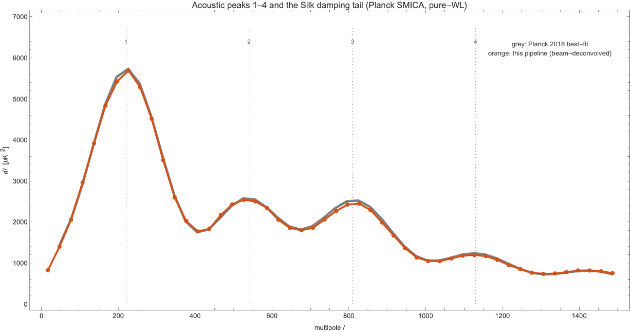
The CMB TT power spectrum from the Planck SMICA map (orange) against the published Planck 2018 best-fit curve (grey). The first four acoustic peaks () and the Silk-damping tail are recovered. Comparing to the smooth best-fit isolates the recovered shape; the scatter of the binned observed Planck points about this curve is cosmic variance.
ℓ≈220,540,810,1130
The mask: f_sky vs MASTER. Masking couples multipoles. The simple correction is leading-order; the rigorous treatment is the MASTER mode-coupling matrix (Hivon et al. 2002), built from the mask power spectrum and Wigner-3j symbols — which we implement from scratch (master.wl). For this large mask the two agree to a few percent:
1
f
sky
M
ℓℓ'
(*fullMASTERdeconvolutiontol=600(seewolfram/master_deconvolve.wls)*)Wl=HealpixSHT`mapToCl[loadSmicaMask[2048],2048,1200];(*maskpowerspectrum*)M=Master`modeCouplingMatrix[Wl,600];(*Wigner-3jcoupling*){ctr,clBins}=Master`masterDeconvolve[cl,M,30,600,25];(*binnedinverse*)(*clBinsagreeswiththef_skyestimate(binnedcl)/fskyto~0.3%*)
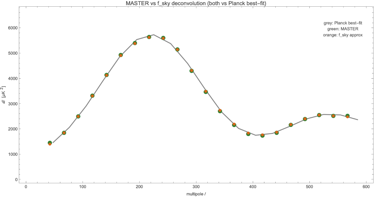
Full MASTER deconvolution (green) vs the approximation (orange), both against the Planck best-fit (grey). For the =0.84 mask they agree closely, confirming the approximation is adequate here.
f
sky
f
sky
5. The acoustic peaks
5. The acoustic peaks
What makes the peaks. Before recombination, photons and baryons were a single fluid. Gravity pulled it into dark-matter potential wells; photon pressure pushed back. The result was standing acoustic oscillations. Modes caught at maximum compression or rarefaction at the moment of recombination show enhanced variance — the peaks. The first peak is the mode that had just time to compress once; its angular scale is a standard ruler (the sound horizon) seen across the whole observable Universe.
We locate the peaks by binning and fitting local parabolas. The recovered positions ≈221,538,803,1099 (for ) match the Planck values (220, 537, 810, 1120) to within the binning resolution.
ℓ
ℓ
n
n=1–4
(*binD_landlocateeachpeakbyalocalparabolafit*)data=Import["cl_smica_ns2048.csv","CSV"][[2;;]];(*ell,Cl_pseudo,Dl_phys*){ll,dd}=Transpose[data[[All,{1,-1}]]];bins=Table[{Mean[#],Mean[dd[[#+1]]]}&@Select[Range[2,1300],lo<=#<lo+25&],{lo,2,1275,25}];{lc,dc}=Transpose[bins];peakIn[lo_,hi_]:=Module[{i=Select[Range@Length@lc,lo<=lc[[#]]<=hi&],f},f=Fit[Transpose[{lc[[i]],dc[[i]]}],{1,x,x^2},x];-Coefficient[f,x]/(2Coefficient[f,x^2])];peaks=peakIn@@@{{140,300},{430,660},{680,920},{980,1280}}(*->{221.,538.,803.,1099.}*)
6. A toy cosmological fit: the acoustic scale
6. A toy cosmological fit: the acoustic scale
The standard ruler. The peak positions are set by one angle, the acoustic scale — the comoving sound horizon at recombination divided by the comoving distance to it:
7. Real-space view: the acoustic ring
7. Real-space view: the acoustic ring
It shows the famously weak correlation at large angles (ℓ > 60°) and the acoustic scale as a feature near ~1°.
Predicted neighbourhood of a hot spot from the measured spectrum: central peak + acoustic cold ring at ~1°.
Acoustic rings under the cursor. Left: a real band-passed SMICA field with the cursor. Middle: the neighbourhood predicted from the measured power spectrum. Right: the actual patch.
You can drag the cursor yourself: evaluate ringExplorer[] (after the Setup cell). The single-patch comparison is deliberately honest — it shows how much signal is hidden in the noise until you stack.
8. The power spectrum in 2D
8. The power spectrum in 2D
9. Position-dependent power: a homogeneity test
9. Position-dependent power: a homogeneity test
Mapping the local small-scale power across the sky (Galactic plane masked) shows it is statistically uniform — the CMB is isotropic:
Local small-scale CMB power per 3.7° patch. Away from the masked Galactic plane it is statistically uniform.
Correlating the two quantities over ~1500 clean patches gives a slope consistent with zero:
10. Conclusions
10. Conclusions
Starting from nothing but the public Planck FITS file and Wolfram Language, we recovered the CMB acoustic peaks and turned the first-peak position into a measurement of a cosmological parameter. The mathematical core — a HEALPix spherical-harmonic transform with a stable Legendre recurrence, and the acoustic-scale distance integrals — is all a few dozen lines of WL, validated against SphericalHarmonicY and a self-consistency round trip.
11. References
11. References
• Planck 2018 results. I & VI. A&A 641 (2020).
• Górski et al., HEALPix, ApJ 622 (2005).
• Hu & Sugiyama, ApJ 471 (1996) — recombination fitting formula.
• Wandelt, Hivon & Górski, MASTER, Phys. Rev. D 64 (2001).
• Chiang, Wandelt et al., position-dependent power spectrum, JCAP 05 (2014) — integrated bispectrum.
• Górski et al., HEALPix, ApJ 622 (2005).
• Hu & Sugiyama, ApJ 471 (1996) — recombination fitting formula.
• Wandelt, Hivon & Górski, MASTER, Phys. Rev. D 64 (2001).
• Chiang, Wandelt et al., position-dependent power spectrum, JCAP 05 (2014) — integrated bispectrum.
Acknowledgement. Based on observations obtained with Planck (http://www.esa.int/Planck), an ESA science mission with instruments and contributions directly funded by ESA Member States, NASA, and Canada. The SMICA map is a product of the Planck Collaboration, obtained from the Planck Legacy Archive.
12. Reproducibility
12. Reproducibility
All code is pure Wolfram Language (one FITS reader, the SHT package, the cosmology package). The only external input is the public Planck SMICA map. See the project repository README for exact commands:
wolframscript -file wolfram/recover_cl.wls 2048 1000 (* recover C_l *)
wolframscript -file wolfram/fit_omega_m.wls 2048 (* peaks + Omega_m *)
wolframscript -file wolfram/fit_omega_m.wls 2048 (* peaks + Omega_m *)
CITE THIS NOTEBOOK
CITE THIS NOTEBOOK
The cosmic microwave background power spectrum from a Planck map
by Marco Thiel
Wolfram Community, STAFF PICKS, June 2, 2026
https://community.wolfram.com/groups/-/m/t/3726129
by Marco Thiel
Wolfram Community, STAFF PICKS, June 2, 2026
https://community.wolfram.com/groups/-/m/t/3726129