Even though the distance between two vertices in the spatial hypergraph is well defined, it is not immediate how this notion of distance may be used as a physical distance measure between objects in space-time. As firstly suggested in [2], the distance between two vertices in the spatial graph reconstructed from the causal graph may be a more similar notion of physical distance instead. In this project I compare these two notions of distance in the Wolfram Model and suggest future ideas to be investigated in this context. Additionally, I highlight and discuss how the size probability of the graph components of the reconstructed spatial graph may follow a power-law distribution for certain rules.
0. Introduction
0. Introduction
At first, the notion of distance in the Wolfram Model [1] seems to be a simple and well defined measure. This is in part true. In fact, the graph distance between two vertices in the spatial hypergraph is well defined and relatively easy to calculate. For instance, using Dijkstra’s algorithm. However, the graph distance in the spatial hypergraph does not immediately correspond to the physical distance that we, beings living in space-time, measure in space-time. As discussed in [2], the vertices in the spatial hypergraph can be seen as “atoms of space” while the edges of the spatial hypergraph represent combinatorial abstract relationships between “atoms of space”.
Definition 1 A “spatial hypergraph, denoted is a finite, undirected hypergraph:
H=(V,E)
E⊂P(V)\{∅}
(
1
)with being the power set of .
P(V)
V
But here is the issue. Supposedly, the hypergraph represents everything in the universe, including all the instruments or objects that we use to measure physical distance (hands, rulers, tapes, digital micrometers, lasers). More in general, the hypergraph should also represents photons, which ultimately are what we use to measure distances in space (and space-time as the speed of light can simply be seen as the proportionality constant between space and time). Since any distance measuring devices is made of collections of "atoms of space" in the hypergraph, when we are measuring the distance between two vertices in the hypergraph we are operating at a far below level of these distance measuring devices [2]. A notion of physical distance in the hypergraph is not so obvious. This project is both an attempt and an invite to discuss this problem further.
1. Causal Graphs and Light Cones
1. Causal Graphs and Light Cones
In modern physics most of the time a distance is measured using photons. This allows us to measure both small and large distances quite precisely. Fundamentally, we simply look at emission and arrival times of photons, i.e., we measure the time between the emission of a photon and when it hits the second detector or bounces off some object. Then, knowing the speed of light, we can convert time into distance (thanks to special relativity the speed of light is constant for all observers). These emission and arrival times can be seen as events in space-time. Obviously, these events are causally related. Here is why this is relevant. As presented in [3, 4], the Wolfram Model introduces a way to construct causal sets algorithmically through the abstract rewriting of edges and vertices in the hypergraph.
Definition 2 [3] An “update rule”, denoted , for a spatial hypergraph , is an abstract rewrite rule of the form -> in which a subhypergraph matching the pattern is replaced by distinct subhypergraph matching the pattern .
R
H=(V,E)
H
1
H
2
H
1
H
2
For instance, the ExampleRule : {{x, y}, {x, z}} -> {{x, z}, {x, w}, {y, w}, {z, w}}, where {{x, y}, {x, z}} = and {{x, z}, {x, w}, {y, w}, {z, w}} = can be represented as
H
1
H
2
In[]:=
ExampleRule = {{x,y},{x,z}}->{{x,z},{x,w},{y,w},{z,w}};RulePlot[ResourceFunction["WolframModel"][ExampleRule]]
Out[]=
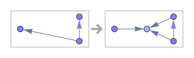
An application of an update rule can be seen as an event.
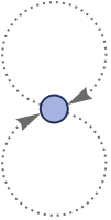
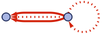
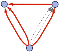
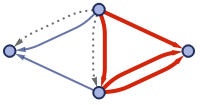
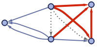
Starting from a initial hypergraph such as {{0,0},{0,0}}, we can see how some rule applications or events may depend on previous ones.
Starting from a initial hypergraph such as {{0,0},{0,0}}, we can see how some rule applications or events may depend on previous ones.
In[]:=
WolframModel[ExampleRule,{{0,0},{0,0}},3]["EventsStatesPlotsList",ImageSize->Tiny]
Out[]=
,
,
,
,
,
,
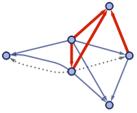
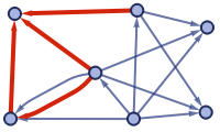
where the edges highlighted in red are the edges created by the rule application. The concept of dependence between rule applications may be formalized as follows by defining a graph which encapsulates the causal relationships between these events.
Definition 3 A Causal Network is a directed acyclic graph in which every vertex corresponds to an application of an update rule (i.e., an event) and in which the directed edge exists iff:
G
causal
A->B
In(B)⋂Out(A)≠∅
(
2
)in other words, if the input for event makes use of hyperedges that were produced by the output of event .
B
A
In Mathematica, this causal graph can be visualized by calling the property LayeredCausalGraph.
In[]:=
SimpleGraph[WolframModel[ExampleRule,{{0,0},{0,0}},3]["CausalGraph",VertexLabels->Automatic,ImageSize->Small]](*SimpleGraph removes multiedges*)
Out[]=
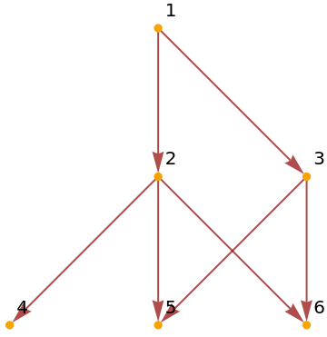
To interpret this, we can see that event 6, which corresponds to the last plot in the EventsStatesPlotsList above, depends on both events 2 and 3 (and obviously event 1 since it is the first event).
If we run the same hypergraph and rule for more generations
In[]:=
ExampleCausal=SimpleGraph[WolframModel[ExampleRule,{{0,0},{0,0}},7]["LayeredCausalGraph",VertexLabels->Automatic]];HighlightGraph[ExampleCausal,Style[Subgraph[ExampleCausal,VertexOutComponent[ExampleCausal, 13]],Red,Thick],ImageSize->Large]
Out[]=
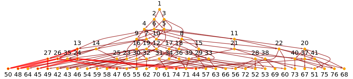
where I have highlighted in Red event 13 and the “causal cone” that it generates, i.e., the set of all vertices in the causal graph causally related to 13.
In the rest of the project, I investigate whether the causal graph may provide a connection between distances in the underlying spatial hypergraph and physical distances.
• Firstly, in Section 2 I summarize the concept of “reconstructed spatial graph” introduced in [2].
• In Section 3 I investigate and provide a visualization of where these events are localized in the underlying spatial graph.
• In Section 4 I define a function to compare distances between spatial hypergraph and reconstructed spatial graph and provide some initial numerical results.
• In Section 5, I discuss the results, further work ideas and conclude the report.
2. Reconstructed Spatial Graph
2. Reconstructed Spatial Graph
As discussed in Section 1, the causal graph may provide a connection between distances in the underlying spatial hypergraph. As introduced in [2], we may attempt to reconstruct the spatial hypergraph using exclusively the information (i.e., vertices and edges) in the causal graph (ExampleCausal above).
The basic idea is to construct a spatial graph using the vertices in the last generation. More in general, we may use vertices in the last foliation but for simplicity in this project I only deal with vertices in the last generation and leave the more general case to be discussed in Section 5.
These vertices are connected if the share a common ancestor in one of the previous updates. For simplicity, I may call this variable ancestorLevel, such that if ancestorLevel = 1 vertices with a common ancestor in the previous generation are connected in the resulting reconstructed spatial graph. If ancestorLevel = 2, vertices with a common ancestor in the last two generations are connected in the reconstructed spatial graph.
I may also define generationNumb to be the total number of generations evaluated.
I may also define generationNumb to be the total number of generations evaluated.
In[]:=
(*Define function used to find the ancestor list of some event in the causal graph*)getAncestorVertexList[g_,event_,ancestorLevel_]:=VertexList[Subgraph[g,VertexInComponent[g,event]]][[Range[1,ancestorLevel+1]]]
In[]:=
ExampleRule = {{x,y},{x,z}}->{{x,y},{x,w},{y,w},{z,w}};generationNumb=7;ExampleWmeo=WolframModel[ExampleRule,Table[{0,0},2],generationNumb];ExampleCausal=ExampleWmeo["LayeredCausalGraph",VertexLabels->Automatic,ImageSize->Full];HighlightGraph[SimpleGraph[ExampleCausal],Style[Subgraph[ExampleCausal,Flatten[{getAncestorVertexList[ExampleCausal,45,1],getAncestorVertexList[ExampleCausal,49,1],getAncestorVertexList[ExampleCausal,46,1]}]],Green,Thick]]
Out[]=
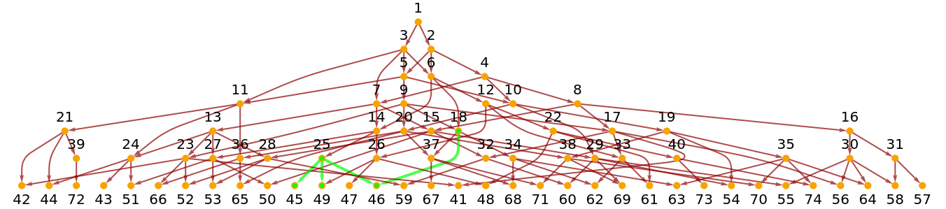
Where I highlight that events 45, 46 and 49 all share a common ancestor in the previous generation. The reconstructed spatial graph will then look like:
In[]:=
(*Function taken from [2]]*)PacletInstall["SetReplace"];<<SetReplace`;SpatialReconstruction[wmo_WolframModelEvolutionObject,dt_Integer:1]:=Module[{cg=wmo["CausalGraph"],ceg=wmo["EventGenerations"],ev0,ev1,oc},ev0=First/@Position[-(ceg-Max[ceg]),dt];ev1=First/@Position[-(ceg-Max[ceg]),0];oc=Select[Rest[VertexOutComponent[cg,#]],MemberQ[ev1,#]&]&/@ev0;Graph[WolframPhysicsProjectStyleData["SpatialGraph","Function"][Graph[ev1,Flatten[(UndirectedEdge@@@Subsets[#,{2}])&/@oc]]],VertexStyle->WolframPhysicsProjectStyleData["CausalGraph","VertexStyle"],EdgeStyle->Blend[{First[WolframPhysicsProjectStyleData["SpatialGraph","EdgeLineStyle"]],WolframPhysicsProjectStyleData["BranchialGraph","EdgeStyle"]}]]]
In[]:=
ancestorLevel=1ReconstructedExample=Graph[SpatialReconstruction[ExampleWmeo,ancestorLevel],VertexLabels->Automatic,ImageSize->Medium]
Out[]=
1
Out[]=
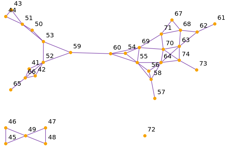
Using ancestorLevel = 2 instead, we obtain:
In[]:=
ancestorLevel=2Graph[SpatialReconstruction[ExampleWmeo,ancestorLevel],VertexLabels->Automatic, ImageSize->Medium]
Out[]=
2
Notice the first big difference. The reconstructed spatial graph obtained using ancestorLevel = 2 is much more connected than that obtained using ancestorLevel = 1. In the latter case, we can identify three components in the reconstructed graph. Obviously, this could have been predicted from causal graph:
One might think this is due to the finite number of generations evaluated and say that, eventually, for a gigantic number of evolutions, the reconstructed spatial graph will have one giant components. As discussed in Section 5, in this example (i.e., for this rule) it is not the case and there may be something more interesting going on (spoiler: it seems that for some rules the probability of the size of the components of the reconstructed spatial graph follows a power-law distribution).
In the reconstructed spatial graph graph distances are also well defined and may be closer to what we mean by physical distance. However, as discussed further in Section 5, there are many assumptions that I have not mentioned. Above all, the choice of foliation was completely arbitrary.
3. Highlight Events in the Spatial Hypergraph
3. Highlight Events in the Spatial Hypergraph
In section 1, I mentioned that the distance between vertices in the underlying spatial graph is well undefined. However, it is not immediate where events are located in the spatial hypergraph. As visualized below, events in the hypergraph can be identified as the set of vertices involved in a rule application.
Below, I define I function that, given the label of a causal graph vertex in the last generation of some WolframModelEvolutionObject outputs the set of spatial hypergraph vertices involved in the rule application event.
Note: this function only works for WolframModelEvolutionObjects with only one rule, for WolframModelEvolutionObjects with a system of rules a more general form of this function is needed. To choose two events from the last generation I defined the following function:
Using these functions, we can highlight vertices in the hypergraph corresponding to some events (as labelled in the causal graph). Here I highlight the vertices in the spatial hypergraph corresponding to events 474 and 420 for the same ExampleWmeo WolframModelEvolutionObject of section 2 but evolved for 10 generations.
In Section 4, to calculate a distance in the spatial hypergraph I select at random one of these vertices and find the path between them.
For purely visualization purposes, we may visually compare the shortest path between events in the spatial hypergraph and the same events in the reconstructed spatial graphs for ancestorLevel = 1 and ancestroLevel= 2:
4. Numerical Work
4. Numerical Work
In this section I provide some numerical results obtained from the comparison of distances between events in the underlying spatial hypergraph and the reconstructed spatial graph.
To calculate and compare distances I defined the following function:
Given a WolframModelEvolutionObject, two events from the last foliation, and the ancestorLevel (see previous sections for the definition of these), the compareDistance function outputs a list with two entries. The first entry is the distance between two events in the spatial hypergraph. The second entry is the distance between the two events in the reconstructed spatial graph for ancestor level = ancestorLevel.
Note: for the compareDistance function to work it needs the functions SpatialReconstruction and fromEventToSpatialVertices to be defined. You can find these functions in the previous sections. Otherwise, since I have used many global variables and functions in the past sections and there may be confusion, in the cells below I collect all the functions and essential variables needed to reproduce results in the rest of this section.
Function Definitions:
Functions:
5. Discussions and Conclusions
5. Discussions and Conclusions
In this section, I provide a discussion of the results and a further investigation of the graph component size when the ancestorLevel = 1.
Result Discussion
Result Discussion
In this project, I have reported the results of some test comparisons between events in the spatial hypergraph and events in the reconstructed spatial graph. The results of tests suggest that, for ancestorLevel = 1 the average distance between events seems to be less in the underlying spatial hypergraph. Results for for ancestorLevel = 2 instead, seem to suggest that the average distance between events seems to be less in the reconstructed spatial graph. Crucially, these results seem to be valid only for WolframModelEvolutionObjects which “look complex”. By “look complex” I mean that no obvious patter can be identified in the respective causal graphs. To be more precise, we can quickly investigate another WolframModelEvolutionObject with the rule
The causal graph, after 4 generations will look like
Trivially, the reconstructed spatial graph will be made of 9 components all of size 3.
In an future extension of this work, similar tests may be conducted using rules that produce “complex” causal graph with no obvious pattern.
In an attempt to formalize this idea of “complexity” of causal graphs mentioned earlier, in the next subsection I show and discuss the probability distribution of the graph component size of the reconstructed spatial graphs.
In an attempt to formalize this idea of “complexity” of causal graphs mentioned earlier, in the next subsection I show and discuss the probability distribution of the graph component size of the reconstructed spatial graphs.
Reconstructed Graph Components
Reconstructed Graph Components
In this subsection I briefly investigate the probability distribution of the graph components size of the reconstructed spatial graph. Similarly as in Section 4 Test 3, it might be interesting to plot the sizes of the various graph components of the reconstructed graph. Here I use the function
Using the same rule as that used in the tests
To be more precise, it is possible to find the empirical probability distribution from the graph components size data
It does look like a power law, investigating a larger graph would probably give better results as well as using a log-bin function.
Conclusion and Further Ideas
Conclusion and Further Ideas
In conclusion, in this project I have compared the distance between two events in the spatial hypergraph and in the reconstructed graph for a specific rule and for a specific kind of foliation. It is important to note that for any other foliation the results are likely to be completely different. The interested reader may explore different rule by simply obtaining some random rules from the Wolfram Rule Registry as follows
and directly use them in this notebook.
Moreover, for the graph distance in the hypergraph to be comparable to a physical distance measured in space-time I have assumed that all edges in the underlying hypergraph are of the same length. This may also not be so obvious. Similarly, different foliations of the causal graph (which effectively may be seen as taking different snapshots of the instantaneous universe) may result in completely different distance relations between events in the reconstructed spatial graph.
As suggested in [2], similar reconstructions of the spatial graph may be adopted. In general, it is possible to reconstruct a spatial graph by using similar relations present in the causal graph. For instance, in this project I have used the common ancestor relation between events. A similar possible relation may be the common successor in the causal graph.
The reader more familiar with the Wolfram Model framework may have noticed the similarities between the reconstructed spatial graph and branchial graphs in multiway systems. Exploring differences and similarities between these two constructions, or perhaps notions of distance in the branchial graphs, may also be interesting ideas to investigate.
To conclude the conclusions, this was only an initial attempt to compare notions of distance in the Wolfram Model formalism. In doing so, the number of questions I have asked definitely outnumber the number of answers I have given here.
Acknowledgments
Acknowledgments
I would like to thank my mentors Nikolay Murzin and Jonathan Gorard for their useful insights and discussions.
References
References
[1] S. Wolfram (2002), A New Kind of Science. Champaign, lllinois: Wolfram Media, Inc. https://www.wolframscience.com
[2] S. Wolfram (2020), Faster than Light in Our Model of Physics: Some Preliminary Thoughts
https://writings.stephenwolfram.com/2020/10/faster-than-light-in-our-model-of-physics-some-preliminary-thoughts/#how-to-measure-distance
https://writings.stephenwolfram.com/2020/10/faster-than-light-in-our-model-of-physics-some-preliminary-thoughts/#how-to-measure-distance
[3] J. Gorard (2020), Algorithmic Causal Sets and the Wolfram Model, arXiv:2011.12174v2
[4] J. Gorard (2020), “Some Relativistic and Gravitational Properties of the Wolfram Model”, Complex Systems 29 (2): 599-654. https://www.complex-systems.com/abstracts/v29_i02_a03/