ABSTRACT (original article): We have derived a series of analytical formulas describing the motion of a nanotip elastically driven across a Gaussian potential well of depth and half width 𝜎. The tip gets pinned if the impact parameter is below a well-defined threshold value. Together with and 𝜎, this value determines the pinning force. The scenario is slightly modified by superimposing a periodic potential with amplitude in the background, provided that ≪. The formulas presented here can be applied to estimate the pinning energy and the linear extension of the perturbation created by a point defect such as an atomic vacancy on a crystal surface from atomic-scale friction force measurements performed by scanning probe microscopy. CITATION (original article): Gnecco, Enrico and Nicolini, Paolo (2024), Atomic-scale stick-slip through a point defect, Phys. Rev. B 109, 134103. https://doi.org/10.1103/PhysRevB.109.134103
𝑈
1
𝑦
0
𝑈
1
𝑈
0
𝑈
0
𝑈
1
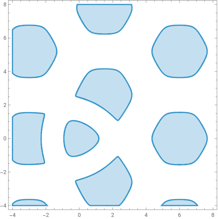
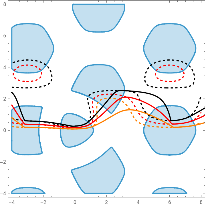
Here we present the derivations leading to Fig. 3 in the original article. We consider a point mass (particle) attached to a spring, the other end of which is driven along a horizontal line with a vertical offset y0. The particle is attracted to the light blue regions (Plot0), corresponding to equilibrium position of the hexagonal potential superimposed to the Gaussian well.
◼
The solid curves (Plot2) represent the actual trajectories of the particle, obtained by solving Newton’s equation numerically for three different offset values.
◼
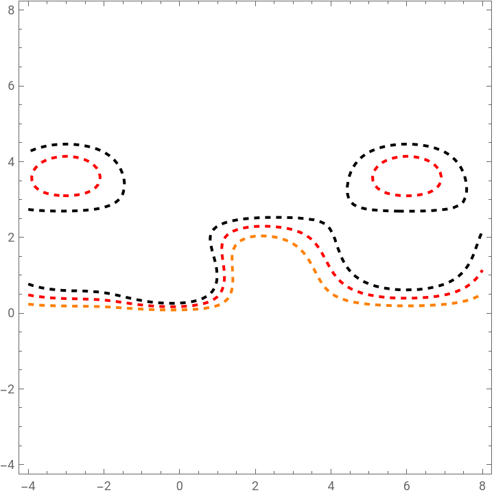
The dashed curves (Plot1) correspond to the associated equilibrium trajectories. These are unstable outside the light blue region => when the particle reaches the boundaries of this region, it is “shot” elsewhere, and meets the dashed curves again within the next stable region.
Mathematica also helped to support the derivation of many equations in the text. In that case, its application is rather straightforward (and it is not presented in this notebook).
Total potential U
In[]:=
U=-U0*(2*Cos[2*Pi*yS/a]*Cos[2*Pi*xS/a/Sqrt[3]+2*Pi/3]+Cos[4*Pi*xS/a/Sqrt[3]+4*Pi/3])-U1*Exp[-(xS^2+yS^2)/2/sigma^2]+U2*Exp[-(xS^2+yS^2)/2/sigma2^2]+(1/2)*k*(xS-x0S-vx*tS)^2+(1/2)*k*(yS-y0S)^2;
First derivatives of U
In[]:=
D1=D[U,xS];D2=D[U,yS];
Second derivatives of U
In[]:=
D11=D[U,xS,xS];D12=D[U,xS,yS];D21=D[U,yS,xS];D22=D[U,yS,yS];
Parameters
m=10^(-5);(*mass*)a=5.2;(*latticeconstant*)gammam=.1;(*dampingcoefficient*)k=1;(*springconstant*)eta=10;(*"Prandtl-Tomlinson"parameter*)x0S=-4;(*startingpoint*)vx=1;(*scanvelocity*)U1=eta;(*attractiveGaussiandepth*)U0=eta/9.1075;(*hexagonallatticecorrugation*)U2=eta/3.7106*0;(*repulsiveGaussiandepth*)sigma=1;(*attractiveGaussianwidth*)sigma2=4.1601;(*repulsiveGaussianwidth*)
Eigenvalues of Hessian
In[]:=
{lambda1,lambda2}=Eigenvalues[{{D11,D12},{D21,D22}}];
Stable equilibrium region
Plot0=RegionPlotlambda1>0&&lambda2>0,{xS,-4,8},{yS,-4,8},
Out[]=
Different offset values
In[]:=
y0List={.8,1.6,2.4};
Stable equilibrium curves
Plot1=ContourPlotEvaluate[Table[D2==0,{y0S,y0List}]],{xS,-4,8},{yS,-4,8},
Out[]=
Trajectories from Newton’ s equation
trajectory[yStartVal_?NumericQ]:=NDSolveValue[{m*x''[t]+gammam*x'[t]==-D1/.{xS->x[t],yS->y[t],tS->t,y0S->yStartVal},m*y''[t]+gammam*y'[t]==-D2/.{xS->x[t],yS->y[t],tS->t,y0S->yStartVal},x[0]==x0S,y[0]==yStartVal,x'[0]==0,y'[0]==0},{x[t],y[t]},{t,0,20}];Plot2=ParametricPlotEvaluate[Table[trajectory[yv],{yv,y0List}]],{t,0,20},(*trajectoriesfromNewton'sequation*)
Out[]=



In[]:=
Show[Plot0,Plot1,Plot2]
Out[]=
CITE THIS NOTEBOOK
CITE THIS NOTEBOOK
Atomic-scale stick-slip through a point defect
by Enrico Gnecco & Paolo Nicolini
Wolfram Community, STAFF PICKS, April 10, 2026
https://community.wolfram.com/groups/-/m/t/3681468
by Enrico Gnecco & Paolo Nicolini
Wolfram Community, STAFF PICKS, April 10, 2026
https://community.wolfram.com/groups/-/m/t/3681468