Abstract:
This work focused on using Mathematica to build a function to compute the microwave spectrum of a broad range of molecules and also implement functions such as Manipulate[], ListPlot[] and Show[] with the aim to improve the visualization process of the rotationally excited energy levels . We create a interactive framework which allows to compute the rovibronic spectrum of a diatomic molecule, as well as the frequencies of its pure rotational transitions and classify those transitions in R Branch and P Branch. Also, we worked on the computing of the rotational frequencies of some triatomic molecules and sorted those values in a Dataset[]. The motivation of this work arises from the need to create an interactive tool that facilitates the analysis of spectroscopic data and allows the effective connection of these results with the theory of molecular structure. Future work aimed at spectroscopy should allow the automated calculation of spectra for any type of molecule.
This work focused on using Mathematica to build a function to compute the microwave spectrum of a broad range of molecules and also implement functions such as Manipulate[], ListPlot[] and Show[] with the aim to improve the visualization process of the rotationally excited energy levels . We create a interactive framework which allows to compute the rovibronic spectrum of a diatomic molecule, as well as the frequencies of its pure rotational transitions and classify those transitions in R Branch and P Branch. Also, we worked on the computing of the rotational frequencies of some triatomic molecules and sorted those values in a Dataset[]. The motivation of this work arises from the need to create an interactive tool that facilitates the analysis of spectroscopic data and allows the effective connection of these results with the theory of molecular structure. Future work aimed at spectroscopy should allow the automated calculation of spectra for any type of molecule.
Introduction
Introduction
One of the biggest challenges in molecular spectroscopy is in interpreting the information obtained about the structure or composition of a molecule. While microwave spectroscopy is a useful tool to determine the isotopic composition of the elements that make up a molecule through analyzing its rotational movements, the interpretation of these spectra is challenging due to how this phenomenon depends on molecular geometry. In order to contribute to this interpretation, this work focuses on using Mathematica and its wide range of functions to calculate and graph rovibrational spectra and thus be used as a learning tool that allows us to more effectively understand the impact of geometry when interpreting spectra. At an academic level, I consider that this type of subject is difficult to teach and learn, since it requires a geometric and dynamic analysis in 3D. Therefore, I am very happy to have been able to work on a project like this that I used Mathematica to meet a challenge such as teaching rotational spectroscopy.
Spectrum of a diatomic molecules
Spectrum of a diatomic molecules
Computing the diatomic molecules spectrum is the most simple case for this kind of problems. To perform this we extract the values of some most commons universal constants using the function SemanticInterpretation[] as follow:
In[]:=
h=SemanticInterpretation["Planck constant value"]//N
Out[]=
In[]:=
sl=SemanticInterpretation["speed of light in m/s"]//N
Out[]=
In[]:=
kb=SemanticInterpretation["Boltzmann Constant value"]//N
Out[]=
“h” is the Planck constant besides we need the value of the speed of light (vacuum) and Boltzmann constant as well.
One of the ways to perform the calculation of these spectra is getting the values of the spectroscopic parameters such as the rotational constants. We used these values reported in a database[1] and set it inside the code .
In[]:=
natureMolecule[1]=pattClF=DispatchℬeQuantity[0.516479,"Centimeters"^(-1)],αeQuantity[0.004357,"Centimeters"^(-1)],eQuantity[786.15,"Centimeters"^(-1)],eeQuantity[6.16,"Centimeters"^(-1)],mp-> ;
In[]:=
natureMolecule[2]=pattHF=DispatchℬeQuantity[20.956,"Centimeters"^(-1)],αeQuantity[0.796,"Centimeters"^(-1)],eQuantity[4138.7,"Centimeters"^(-1)],eeQuantity[90.0,"Centimeters"^(-1)],mp ;
In[]:=
natureMolecule[3]=pattICl=DispatchℬeQuantity[0.1141587,"Centimeters"^(-1)],αeQuantity[0.0005354,"Centimeters"^(-1)],eQuantity[384.293,"Centimeters"^(-1)],eeQuantity[1.501,"Centimeters"^(-1)],mp ;
In[]:=
natureMolecule[4]=pattCO=DispatchℬeQuantity[1.93127,"Centimeters"^(-1)],αeQuantity[0.01751,"Centimeters"^(-1)],eQuantity[2169.8,"Centimeters"^(-1)],eeQuantity[13.294,"Centimeters"^(-1)],mp ;
In[]:=
natureMolecule[5]=pattBrF=DispatchℬeQuantity[0.35584,"Centimeters"^(-1)],αeQuantity[0.00261,"Centimeters"^(-1)],eQuantity[670.75,"Centimeters"^(-1)],eeQuantity[4.054,"Centimeters"^(-1)],mp ;
In[]:=
natureMolecule[6]=pattHCl=DispatchℬeQuantity[10.59341,"Centimeters"^(-1)],αeQuantity[0.30718,"Centimeters"^(-1)],eQuantity[2990.946,"Centimeters"^(-1)],eeQuantity[52.8186,"Centimeters"^(-1)],mp ;
where each of these parameter mean
◼
ℬe is the rotational constant evaluated only in the equilibrium position of diatomic molecule
◼
e is the equilibrium vibration frequency under the harmonic approximation of diatomic molecule
◼
is the vibrational quantum number
◼
J is the rotational quantum number
◼
αe is the vibration - rotation coupling constant
◼
v is the inertial distortion constant
◼
ee
Once, with all the parameters loaded we used the Manipulate[] and Module[] functions to generate a interactive framework that contains all the equations derivate from Quantum Mechanics that allow simulating this kind of molecular systems.
In[]:=
ManipulateModule{ℰrot,partiFunRot,popRot,rovibEnergy,frequencyRot,frequencyP,frequencyR,microwavelines,peaksP,peaksR,spectrumR,spectrumP,frequencyTable},ℰrot[J_,_,ℬe_,αe_,e_]:=ℰrot[J,,ℬe,αe,e]=ℬe-αe+J(J+1)-slh;partiFunRot[J_,_,ℬe_,αe_,e_,T_]:=Sum(2j+1)ExpQuantityMagnitude@,{j,0,10,1};popRot[J_,_,ℬe_,αe_,e_,T_]:=;rovibEnergy[J_,_,ℬe_,αe_,e_,ee_]:=e+-ee+ℬe-αe+J(J+1)-;frequencyRot[J_,_,ℬe_,αe_,e_]:=2(J+1)ℬe-αe+-4;frequencyP[J_,_,ℬe_,αe_,e_,ee_]:=rovibEnergy[J-1,+1,ℬe,αe,e,ee]-rovibEnergy[J,,ℬe,αe,e,ee];frequencyR[J_,_,ℬe_,αe_,e_,ee_]:=rovibEnergy[J+1,+1,ℬe,αe,e,ee]-rovibEnergy[J,,ℬe,αe,e,ee];microwavelines=Table[{(frequencyRot[J,0,ℬe,αe,e]/.natureMolecule[k])sl,popRot[J,0,ℬe,αe,e,T]/.natureMolecule[k]},{J,0,10,1}];frequencyTable=MapAt[UnitConvert[#,"Megahertz"]&,Table[{J,J-1,microwavelines〚J,1〛},{J,1,11,1}],{All,3}];peaksP=Table[{frequencyP[J,0,ℬe,αe,e,ee]/.natureMolecule[k],J(popRot[J,0,ℬe,αe,e,T]/.natureMolecule[k])},{J,1,20,1}];peaksR=Table[{frequencyR[J,0,ℬe,αe,e,ee]/.natureMolecule[k],(J+1)(popRot[J,0,ℬe,αe,e,T]/.natureMolecule[k])},{J,0,20,1}];spectrumR=MapIndexed[{#2〚1〛-1,#1〚1〛}&,peaksR];spectrumP=MapIndexed[{#2〚1〛,#1〚1〛}&,peaksP];Grid[{{Show[ListPlot[peaksR,PlotRange{{Min[peaksP〚;;,1〛],Max[peaksR〚;;,1〛]},All},FillingAxis,ImageSizeMedium,PlotStyleWhite,FillingStyleRed,FrameTrue,FrameLabel{"Wavenumber ()","Population"},PlotLabelStyle["Rovibronic spectrum"],PlotLegendsRow[{Red," R Branch"}]],ListPlot[peaksP,PlotRange{{Min[peaksP〚;;,1〛],Max[peaksR〚;;,1〛]},All},FillingAxis,ImageSizeMedium,PlotStyleWhite,FillingStyleBlue,FrameTrue,FrameLabel{"Wavenumber ()","Population"},PlotLabelStyle["Rovibronic spectrum"],PlotLegendsRow[{Blue," P Branch"}]]],mp/.natureMolecule[k]},{Labeled[Dataset[{<|"R Branch"{<|MapThread[Rule,{{"J","Frequency"},#}]|>&/@spectrumR},"P Branch"{<|MapThread[Rule,{{"J","Frequency"},#}]|>&/@spectrumP}|>}],Style["Rovibronic Spectrum lines","Text"],Top],Labeled[Dataset[<|MapThread[Rule,{{"J'","J","Frequency"},#}]|>&/@frequencyTable],Style["Rotational Pure Transitions","Text"],Top]}}],Control[{{k,4,"Molecule:"},{1"ClF",2"HF",3"ICl",4"CO",5"BrF",6"HCl"},Setter}],Control[{{T,150,"Temperature (K)"},150,300,50}]
1
2
4
3
ℬe
2
e
2
J
2
(J+1)
-ℰrot[j,,ℬe,αe,e]
kbT
ExpQuantityMagnitude@
-ℰrot[J,,ℬe,αe,e]
kbT
partiFunRot[J,,ℬe,αe,e,T]
1
2
2
+
1
2
1
2
4
3
ℬe
2
e
2
J
2
(J+1)
1
2
4
3
ℬe
2
e
3
(J+1)
-1
cm
-1
cm
Out[]=
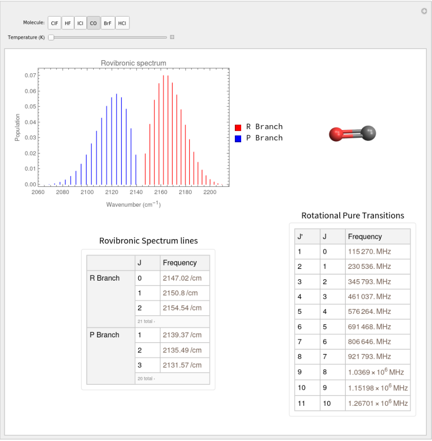
Above, we can see that there is a lot of information showed as:
◼
The MoleculePlot3D[] of the respectively diatomic molecule
◼
The Rovibronic spectrum of the molecule (Reds bars are the R branches transitions and the blue ones are the P branches), here we used ListPlot[] and Show[] functions to plot the spectrum
◼
The frequencies of the pure rotational transitions (neglecting the vibrational interactions) are listed as a Dataset[]
◼
The frequencies of the rovibronic spectrum are listed
Using the control panel inside of the Manipulate[] function you can control the temperature variable and change the nature of the molecule as well, you will see the above results respectively for each chosen molecule.
Triatomic Linear molecules
Triatomic Linear molecules
The triatomic system is similar to diatomic but in this case, the fact to added another atom increases the magnitude of the interaction between rotations and vibrations. Therefore, the number of the spectroscopic parameters changes but we set up in the code as follow:
Now, the selected molecule is HCN.
Similarly to the previous section, we created a interactive framework in which the nature of the triatomic molecule is changing but here only the tables with the frequencies of rotational transitions are displayed.
Other project insights
Other project insights
Throughout the development of the project, a lot of work was done on the automatic handling of physical units by Mathematica. In addition, emphasis was placed on the automatic extraction of universal constant values and the use of the Dataset[] function to organize the data that was obtained.
Future work
Future work
This is just the beginning, there are a lot of work to be done around the molecular spectroscopy. As a suggestion, the next step would be to compute (create an automatic algorithm) all these spectroscopic constants performing quantum mechanics calculations with the aim of improving the accuracy of the data and be able to compute all spectra of any molecule.
In conclusion, this project demonstrated a way to employ Mathematica to study and visualize spectroscopic topics. In my personal opinion, this is a potential tool to be implemented in the academic undergraduate courses and with further improvements this can be employed for an outstanding research project .
References
References
◼
[1]National Institute of Standards And Technology , Chemistry web book NIST Link: https://webbook.nist.gov/chemistry/form-ser/ (Last revision July 12th 2020)
◼
[2]P. Kisliuk, C.H. Townes, “Molecular Microwave Spectra Tables”, National Bureau of Standars, Vol. 44, 611 p. 1950.
◼
[3]C.H. Townes, A.L. Schwalow, “Microwave Spectroscopy” McGraw-Hill , New York.
◼
[4]Ira. N. L, “Molecular Spectroscopy” John Wiley & Sons, Inc .1975
◼
[5]P.W. Atkins, R.S. Friedman,“Molecular Quantum Mechanics” Third Edition,1996
◼
[6]G.Hezberg, “Molecular Spectra and Molecular Structure I” Princeton, New Jersey,1950