This notebook summarizes the exploration and analysis of ordinary differential equations (ODEs) using symbolic computation. The focus is on solving first-order ODEs, where the rate of change of a function is defined in relation to and itself, such as x and sin(y) . By applying initial conditions e.g., , unique solutions are determined, illustrating the concept of initial value problems in differential equations.Using the Wolfram Language, explicit solutions to these ODEs are derived, followed by graphical representations to visualize the function y(x) over specified intervals. This process not only aids in understanding the mathematical solutions but also in interpreting the system dynamics modeled by the equations.The notebook extends to identifying equilibrium points in differential equations, signifying states where the system experiences no net change, thus highlighting the steady-state behavior. This exploration showcases the integration of symbolic computation in solving and analyzing mathematical models, particularly emphasizing the utility and power of computational tools in understanding complex systems governed by differential equations.
y(x)
x
y
dy
dx
dy
dx
y(0)3
Example 1
Example 1
dy
dx
In[]:=
gsol=DSolve[y'[x]==x,y[x],x]
Out[]=
y[x]+
2
x
2
1
In[]:=
psol=Simplify[DSolve[{y'[x]==x,y[0]==3},y[x],x]]
Out[]=
y[x](6+)
1
2
2
x
In[]:=
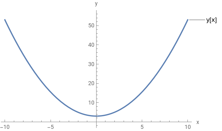
solutionPlot=Plot[Evaluate[y[x]/.psol],{x,-10,10},PlotLabels->"y[x]",AxesLabel->{"x","y"}]
Out[]=
In[]:=
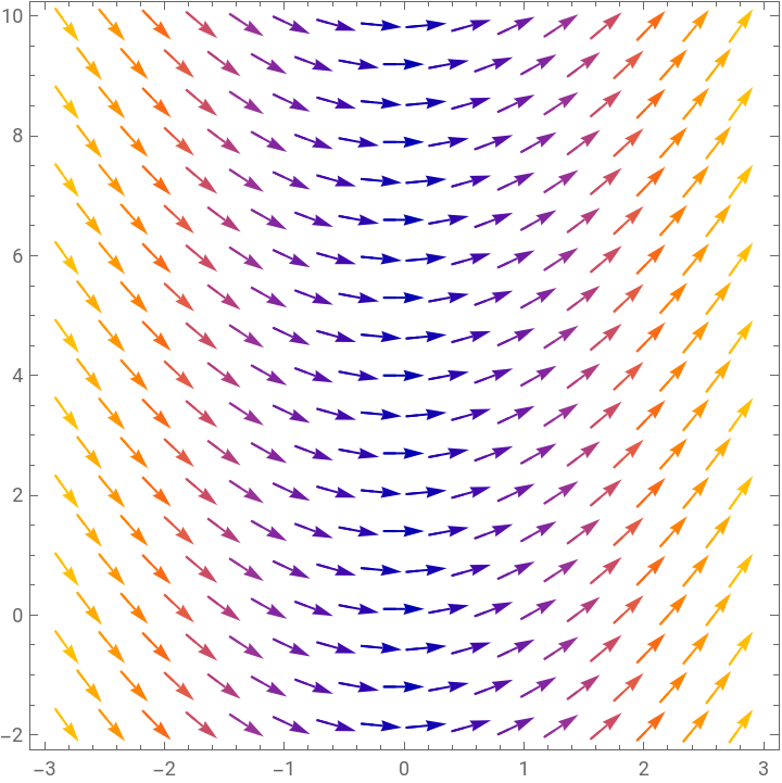
slopeField=VectorPlot[{1,x},{x,-3,3},{y,-2,10}]
Out[]=
In[]:=
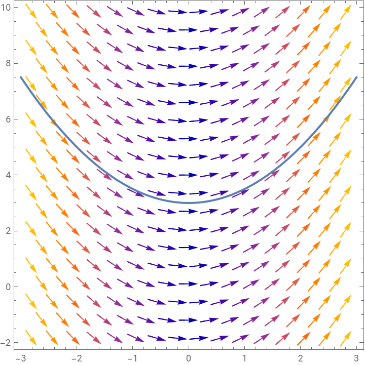
Show[slopeField,solutionPlot]
Out[]=
Example 2
Example 2
In[]:=
Clear["Global`*"]
In[]:=
x-y,y(0)0
dy
dx
In[]:=
gsol=DSolve[y'[x]==x-y[x],y[x],x]
Out[]=
{{y[x]-1+x+}}
-x
1
In[]:=
psol=Simplify[DSolve[{y'[x]==x-y[x],y[0]==0},y[x],x]]
Out[]=
{{y[x]-1++x}}
-x
In[]:=
solutionPlot=Plot[Evaluate[y[x]/.psol],{x,-5,10},PlotLabels->"y[x]",AxesLabel->{"x","y"}]
Out[]=
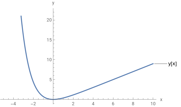
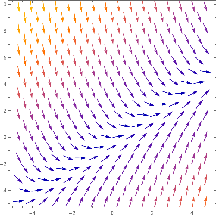
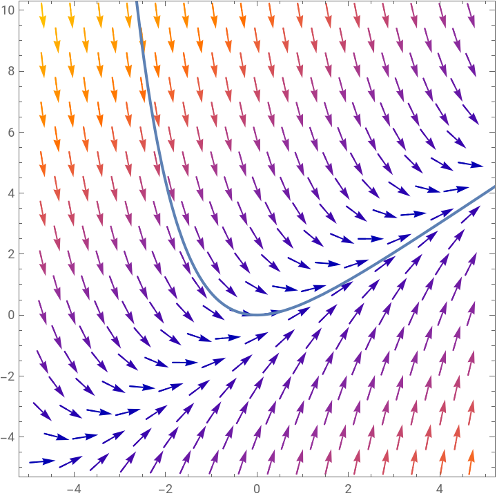
If we look at the slope field we can see that from both directions all of the slopes are kind of swooping into one diagonal line here. We call this diagonal line an isocline.
In[]:=
slopeField=VectorPlot[{1,x-y},{x,-5,5},{y,-5,10}]
Out[]=
In[]:=
Show[slopeField,solutionPlot]
Out[]=
Example 3
Example 3
This is called a repeller
Example 4
Example 4
Example 5
Example 5