This project aims to simulate the ground state of hydrogen-like atoms using quantum computing tools in Mathematica. It employs quantum circuits to represent fermionic operators, following the principles of Hartree-Fock theory. By applying mixed Quantum-Classical algorithms like the Variational Quantum Eigensolver, the goal is to minimize energy within the circuits, thereby transforming initial states into the ground state of a Hartree-Fock Hamiltonian. This research demonstrates the potential of quantum computing in simulating atomic structures and computational chemistry.
Helium atom as a quantum circuit
Helium atom as a quantum circuit
Creating computational basis for the problem
Creating computational basis for the problem
Required imports and global variables
Required imports and global variables
First we shell import required packages. We will use Wolfram Quantum Framework to simulate quantum circuits and quantum states.
In[]:=
Needs["Wolfram`QuantumFramework`"];Needs["Wolfram`QuantumFramework`ExampleRepository`"]
In second step we define global variables. NChannels represents number of orbitals that one wants to use to simulate the atom. In general the more the better. One needs to however keep the number of channels low since they are mapped later to qubits. Large numbers of qubits are in general hard to simulate on classical computer. Z=2 stands for atomic number of Helium. Variable e0 is ground state energy of Helium in Hartrees.
In[]:=
NChannels=4;Z=2;e0=-0.5;init=ConstantArray[0,3NChannels];init=ReplacePart[init,{1->π,2->π}]
Hydrogen-like states in Fock Basis
Hydrogen-like states in Fock Basis
To simulate simple atoms we can use one-to-one correspondence of electron algebra with qubit algebra. We define each qubit as representation of hydrogen-like orbital. Let us use 4 orbitals (two 1s and two 2p) for the sake of this Helium atom calculation.
In[]:=
tableOfStates=Flatten[#,3]&[Table[{n->nIter,l->lIter,m->mIter,ms->msIter},{nIter,1,Quotient[NChannels,2]+1},{lIter,0,nIter-1},{mIter,-lIter,lIter},{msIter,-1/2,1/2,1}]];tableOfStates=Take[tableOfStates,NChannels];TableForm[#,TableHeadings->{Range[tableOfStates//Length],None}]&[tableOfStates]
Out[]//TableForm=
1 | n1 | l0 | m0 | ms- 1 2 |
2 | n1 | l0 | m0 | ms 1 2 |
3 | n2 | l0 | m0 | ms- 1 2 |
4 | n2 | l0 | m0 | ms 1 2 |
Hartree integrals
Hartree integrals
General Hartree-Fock hamiltonian can be described in Fock basis in the form:
H=+,
N
∑
i,j=0
h
ij
†
a
i
a
j
1
2
N
∑
i,j,k,l=1
h
ijkl
†
a
i
†
a
j
a
k
a
l
where
h
ij
*
ϕ
i
2
p
2m
ϕ
j
h
ijkl
dτ
1
dτ
2
*
ϕ
i
*
ϕ
j
ϕ
k
ϕ
l
are hartree integrals. In the case of Helium atom is diagonal for hydrogen-like orbitals and it’s value is = where n is principal quantum number. Two body potential is given by the formula . Our choice of basis orbital functions is to make the problem clear in terms of physical meaning of the transition terms etc. It is however not the best in terms of computation. Orbital two-body integrals in hydrogen basis give accurate values for transition probability. Although accurate, they are numerically heavy. One may take other basis’ into consideration such as STO-3g etc. Hydrogen-like integrals can be computed semi-analytically. The integration is cumbersome and can be found in the Appendix.
h
ij
h
nn
2
Z
E
0
2
n
V(r-r')=
1
|r-r'|
This bit of code takes up to 2 minutes to compute .
In[]:=
Y[{li_?IntegerQ,mi_?IntegerQ},{lh_?IntegerQ,mh_?IntegerQ},{lj_?IntegerQ,mj_?IntegerQ},{lk_?IntegerQ,mk_?IntegerQ},{l_?IntegerQ,m_?IntegerQ}]:=Sqrt[]ClebschGordan[{l,0},{lk,0},{lh,0}]ClebschGordan[{l,m},{lk,mk},{lh,mh}]ClebschGordan[{l,0},{lj,0},{li,0}]ClebschGordan[{l,-m},{lj,mj},{li,mi}];
m
(-1)
2lk+1
2lh+1
2lj+1
2li+1
In[]:=
Rad[n_?IntegerQ,l_?IntegerQ,r_]:=Sqrt[Factorial[n+l]]Exp[-Z]LaguerreL[n-l-1,2l+1,(2Z)];
ZFactorial[(n-l-1)]
2
n
r
n
l+1
(r)
2Z
n
r
n
1
r
In[]:=
R[{ni_?IntegerQ,li_?IntegerQ},{nh_?IntegerQ,lh_?IntegerQ},{nj_?IntegerQ,lj_?IntegerQ},{nk_?IntegerQ,lk_?IntegerQ},l_?IntegerQ]:=NIntegrate[x^2Rad[ni,li,x]Rad[nj,lj,x]*(1/x^(l+1)Integrate[Rad[nh,lh,y]Rad[nk,lk,y]y^(l+2),{y,0,x}]+Integrate[Rad[nh,lh,y]Rad[nk,lk,y]/y^(l-1),{y,x,∞}]),{x,0,∞}];
l
x
In[]:=
Hartree[{ni_?IntegerQ,li_?IntegerQ,mi_?IntegerQ},{nh_?IntegerQ,lh_?IntegerQ,mh_?IntegerQ},{nj_?IntegerQ,lj_?IntegerQ,mj_?IntegerQ},{nk_?IntegerQ,lk_?IntegerQ,mk_?IntegerQ}]:=Module[{i,f},i=Max[Abs[lk-lh],Abs[li-lj]];f=Min[lk+lh,li+lj];Sum[If[Y[{li,mi},{lh,mh},{lj,mj},{lk,mk},{l,m}]==0,0,Y[{li,mi},{lh,mh},{lj,mj},{lk,mk},{l,m}]*N[R[{ni,li},{nh,lh},{nj,lj},{nk,lk},l]]],{l,i,f},{m,-l,l}]];
In[]:=
sStates=Table[{i,j,k,l}->Hartree[{i,0,0},{j,0,0},{k,0,0},{l,0,0}],{i,1,2},{j,1,2},{k,1,2},{l,1,2}]//ArrayFlatten//Flatten//Association
Out[]=
{1,1,1,1}1.25,{1,1,1,2}0.17871,{1,2,1,1}0.17871,{1,2,1,2}0.419753,{1,1,2,1}0.17871,{1,1,2,2}0.0438957,{1,2,2,1}0.0438957,{1,2,2,2}0.0171633,{2,1,1,1}0.17871,{2,1,1,2}0.0438957,{2,2,1,1}0.0438957,{2,2,1,2}0.0171633,{2,1,2,1}0.419753,{2,1,2,2}0.0171633,{2,2,2,1}0.0171633,{2,2,2,2}0.300781
Defining the problem as a quantum circuit
Defining the problem as a quantum circuit
Computational ansatz
Computational ansatz
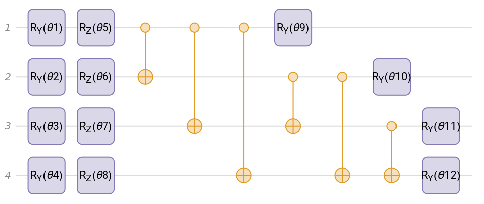
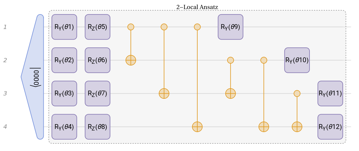
To conduce any variational method computation we need a state ansatz. In the case of quantum computing the ansatz is a quantum circuit that is controllable and transforms series of qubit 0’s to arbitrary vector in Hilbert space. For this calculation we chose to use the truncated two-local ansatz. It consists of four gate layers. First and second layers are parametrized rotations on Bloch sphere over Y and Z axes subsequently. These layers generate arbitrary non-entangled state. Next we have a sequence of CNOT gates that aim to entangle the state created in the first two layers. Finally we transfer this state to different basis. Originally it is achieved by using two rotations over X and Y axis. We chose to truncate the last layer. The ansatz can be thought of as a state that is first prepared in basis A, then entangled and measured in the basis B.
In[]:=
Options[parametrizedLayer]={"Symbol"->"θ"};parametrizedLayer[op_,range_List,OptionsPattern[]]:=Sequence@@Table[op[Symbol[OptionValue["Symbol"]<>ToString[i]]]->Flatten[Position[range,i]],{i,range}]
parametrizedLayer["RY",Range[NChannels+1,2NChannels]];
In[]:=
entaglementLayer[cop_,range_List]:=Sequence@@Thread[cop->Subsets[Range[NChannels],{2}]]
entaglementLayer["CNOT",Range[NChannels]];
In[]:=
NLayers=3;
In[]:=
params=Table[Symbol["θ"<>ToString[i]],{i,1,NLayers*NChannels}]
Out[]=
{θ1,θ2,θ3,θ4,θ5,θ6,θ7,θ8,θ9,θ10,θ11,θ12}
In[]:=
ansatz=QuantumCircuitOperator[{parametrizedLayer["RY",Range[NChannels]],parametrizedLayer["RZ",Range[NChannels+1,2NChannels]],entaglementLayer["CNOT",Range[NChannels]],parametrizedLayer["RY",Range[1+2NChannels,3*NChannels]]},"Parameters"->params,"Label"->"2-Local Ansatz"];
In[]:=
ansatz["Diagram"]
Out[]=
In[]:=
stateAnsatz=ansatz[];
In[]:=
QuantumCircuitOperator[{StringRepeat["0",NChannels],ansatz}]["Diagram"]
Out[]=
Jordan-Wigner transformation of a Hamiltonian
Jordan-Wigner transformation of a Hamiltonian
To obtain the computational hamiltonian we need to transform fermionic creation and annihilation operators acting on atomic orbitals to sequence of gates acting on computational qubits. The method of doing this is called Jordan-Wigner transformation [5]:
Hamiltonian as a quantum circuit
Hamiltonian as a quantum circuit
Hamiltonian as a non-unitary operator doesn’t have trivial quantum circuit representation. One needs to use some method to simulate it. For the sake of this computation we used a method of decomposing hamiltonian into sum of tensor products of Pauli gates. Then we compile a multiplexer to create a sum weighted by the ancilla qubits. We start with the definition of Hartree hamiltonian in computational basis (the computation may take up to two minutes):
We decompose the hamiltonian in the Pauli basis and truncate small terms as they result from computational errors.
To compile the whole circuit we need to add the ansatz circuit in the beginning and inversed ansatz at the end. Such circuit computes the expected value of energy.
We can extract the energy expectation value using ComplexExpand[]
Energy Search
Energy Search
Cost function
Cost function
We can define energy expectation value to be the cost function for the optimization algorithm. We will use the Natural gradient descent.
Gradient descent
Gradient descent
To conduce a successful search of energy minimizing parameters we need to use the Fubini metric. The mapping between the parameter space of the ansatz and target Hilbert space is not isometric. We therefore should use the study metric. The gradient operator guides us downhill in the direction minimizing the energy. The Fubini study metric makes sure we we walk carefully and don’t take too large steps.
The resulting energy is quite far from the known value for Helium. We can plot the amplitudes for different states.
Concluding Remarks
Concluding Remarks
The presented method is suitable for many qubit, error corrected quantum computers. It is then not possible to use it for computation as for now. There are also problems with growing complexity of the circuit. Although we reduce the dimension of the parameter space from exponential to linear, we trade it of with quadratic growing complexity of CNOT layer of the ansatz. Additionally, current mapping of the hamiltonian grows exponentially in terms of circuit complexity. This growth can be suppressed by the truncation of Pauli gates with small weights. For atomic systems it may be however not sufficient because of strong interactions of electron clouds and thus emerging strong correlations. The method is nonetheless suitable for quantum chemistry simulations where one can take into account valence band electrons distributed over many atoms.
The notebook can serve as a demonstration of possibilities of Wolfram Quantum framework. In particular it may serve as an instruction on how to create general classes of quantum circuits simulating atomic electron configurations.
Acknowledgments
Acknowledgments
I would like to thank my mentor Mads Bahrami for introducing me to the topic of quantum chemistry simulations using quantum circuits. I’d also like to thank my other mentor Paul Abbott for all theoretical insight in Helium atom simulations. I would like to thank my Teaching Assistants Sebastian Rodriguez and Bruno Tenorio for their priceless help in finding errors in my code and tunneling through all of the conceptual difficulties and Payal Solanki for providing knowledge about how to construct computational ansatze. Finally, I would like to thank professor Stephen Wolfram for keeping an eye on my progress during the summer school.
References
References
1
.Bethe and Salpeter (1957), Quantum Mechanics of One and Two Electron Atoms. Springer-Verlag.
2
.Abbott and Malsen (1986), A model wavefunction including electron correlation for the
ground state of the helium isoelectronic sequence. J. Phys. B: At. Mol. Phys. 19.
ground state of the helium isoelectronic sequence. J. Phys. B: At. Mol. Phys. 19.
3
.Tilly et al. (2022), The Variational Quantum Eigensolver: a review of methods and
best practice arxiv.org/pdf/2111.05176.
best practice arxiv.org/pdf/2111.05176.
4
.Whitfield et al. (2010), Simulation of Electronic Structure Hamiltonians Using
Quantum Computers. arxiv.org/pdf/1001.3855.
Quantum Computers. arxiv.org/pdf/1001.3855.
Cite This Notebook
Cite This Notebook